Dot Density Map: Mapping Distribution With Dots
 By Tony Astor ·

Dot Density Map
A dot density map places one dot for every fixed count of a phenomenon, such as one dot per 100 people, so densely packed dots reveal hot spots and sparse dots show low concentration. Because each dot represents a constant value, density communicates intensity directly, exposing internal geography that uniform polygon shading hides.
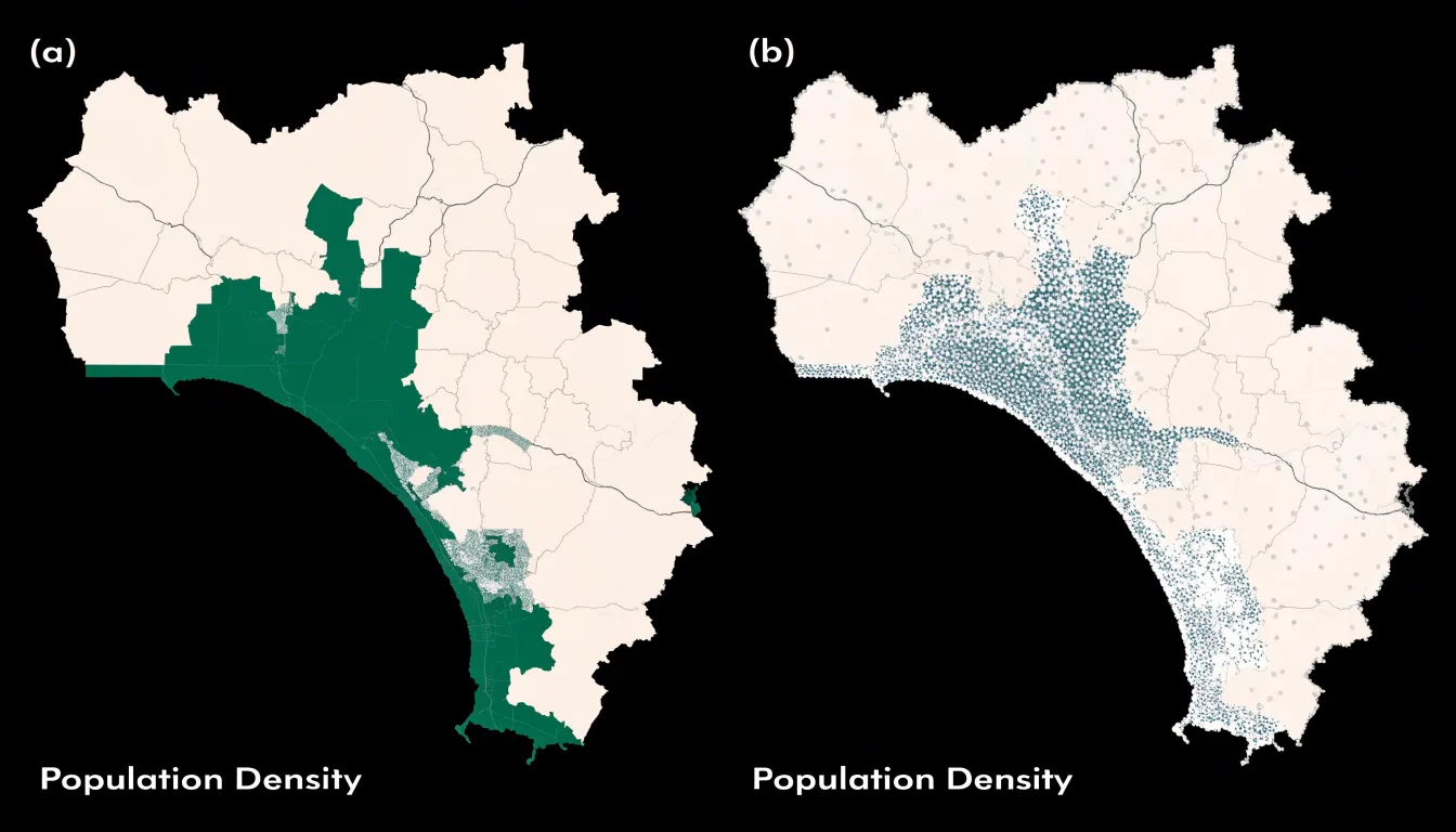
Table of Contents
- Dot Density Map
- Dot Scale
- Dot Placement
- Dot Size
- Dot Color
- Pattern Recognition
- Common Misreadings
- Population Distribution
- Wildlife and Environmental Tracking
- Business Location Intelligence
- Choropleth vs. Dot Density
- Data Preparation
- Interactive and Mobile Mapping
- Ethical Mapping
- Map Design Checklist
Dot Density Map
A dot density map places one dot for every fixed count of a phenomenon, spreading thousands of marks across a geographic area so the eye reads raw concentration directly. Where dots pile up densely, a hot spot announces itself; where they thin out, the viewer sees sparsity. This visual grammar lets patterns emerge from the data rather than from the administrative units drawn around them.
A single large polygon colored a uniform shade can hide the fact that most of its residents cluster along a river corridor while the rest of the territory sits nearly empty. Dot concentration restores that internal geography, showing gradients from crowded cores to quiet peripheries and exposing regional variances that boundary shading flattens into one tone. Readers can trace the shape of a hot spot, follow a corridor of activity, and compare the texture of one district against another at a glance.
Because each dot represents a constant value, doubling the dots doubles the count, and mark density communicates intensity without requiring a legend for every shade. The technique works especially well for population, housing, crop acreage, or incidents, where the underlying distribution is uneven and clustered. Boundaries still provide reference, yet they recede into context while the dots show where values are concentrated and where activity thins away.
Dot Scale
The dot scale defines the unit value that each individual dot represents—for example, one dot standing in for 100 people—and directly determines how many symbols appear on the canvas. A low value such as one dot per person produces an enormous number of symbols in densely settled areas, merging into solid blocks of ink that conceal the underlying pattern. A high value reduces the symbol count but begins to distort the picture, since small concentrations may be rounded away entirely and the map starts to understate real differences between places.
Selecting a good value begins with the densest area the map must show. Calculate how many dots that area would generate at a candidate scale and check whether the resulting symbols can still be distinguished from one another. As a working rule, the busiest region should remain legible as a field of separate dots rather than a filled polygon. Because scale effects are difficult to predict in the abstract, test several values and compare the resulting maps side by side.
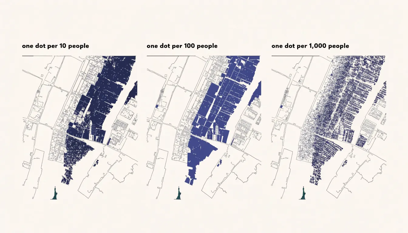
The scale should also match the map’s geographic scope and total population. A national map covering tens of millions of people needs a larger unit value than a city map, because the same dot count spread across a smaller area reads differently. Round numbers such as one dot per 50, 100, or 1,000 make the legend easy to grasp and allow readers to estimate quantities by counting small groups of symbols. State the chosen value plainly in the legend and keep it consistent across any series of maps so comparisons between them remain valid.
Dot Placement
Dot placement hinges on whether dots represent exact locations or are distributed randomly within administrative boundaries:
- Exact placement: Dots are placed at precise geocoded coordinates, such as a street address or a GPS point. The spatial arrangement directly reflects the underlying data, allowing viewers to discern fine-scale patterns like clusters along roads or within neighborhoods. However, exact placement requires highly granular data, which is often unavailable or unreliable due to privacy concerns, incomplete records, or geocoding errors.
- Random distribution: Algorithms use a uniform random process to scatter dots within administrative polygons, such as census tracts or counties, matching the aggregated count for that area. This preserves the overall density pattern while obscuring individual locations to protect confidentiality. Because dots are spread evenly across each polygon, the resulting map is smoother and less precise, which can smooth out local variations and mislead viewers about actual clustering.
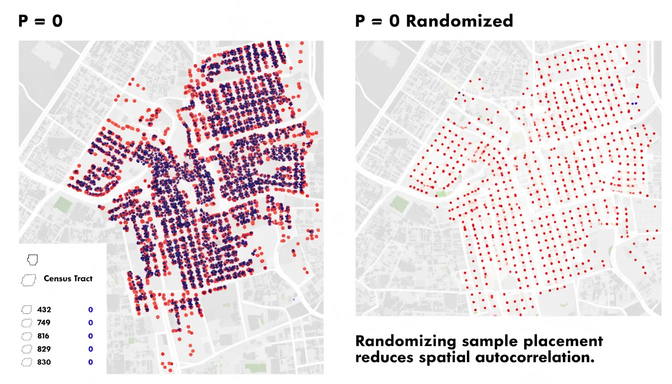
The choice between exact and random placement depends on whether point-level or only aggregate data are available, and on the balance between revealing micro-scale patterns and protecting privacy.
Dot Size
The pixel radius of a single dot determines how much ink lands on the canvas and how legible each mark stays at normal viewing distance. A radius that is too large causes neighboring dots to overlap into solid blocks, producing visual noise that obscures the pattern. A radius that is too small leaves dots as isolated specks that are difficult to see, particularly on smaller screens or in print.
Calibrating the pixel radius requires balancing data density against the physical dimensions of the map. A radius suited to sparse rural regions can quickly saturate a dense city center. Test several candidate radii against the map’s densest area, then select the largest value that still preserves visible white space between individual dots in that region. This keeps the densest zones readable while giving sparser areas enough visual weight to register.
Rendering choices also interact with dot size. Anti-aliasing softens edges and can make smaller dots appear hazy, while fully opaque circles at larger radii dominate the composition. A moderate radius—often in the range of two to four pixels depending on output resolution—balances crispness with restraint.
Dot Color
Color allows a dot density map to carry more than one category of information at once. By assigning a distinct hue to each group, a single map can show where several populations or land uses occur and how they intermingle. In demographic mapping, different colors might represent separate age brackets distributed within their respective boundaries, revealing clustering, segregation, and overlap that separate single-category maps would obscure. Similarly, land-use maps can distribute residential, commercial, industrial, and recreational dots across a region to show development textures and transitions between zones.
Effective categorical color coding depends on several practical rules:
- Choose hues that remain distinguishable at small sizes and hold up when dots sit close together or overlap.
- Limit the number of categories so viewers can match colors to the legend without effort.
- Adjust dot size and opacity so dense clusters do not obscure individual colors or blur boundaries between groups.
- Where categories are numerous, use a consistent, well-ordered legend to help readers decode the pattern quickly.
Pattern Recognition
When viewing a dot density map, the human visual system automatically groups nearby dots and perceives clusters, gradients, and empty spaces. Rooted in Gestalt principles of proximity and similarity, this parallel processing extracts meaning from the overall spatial configuration before the viewer focuses on individual points. A dense cluster of housing dots immediately signals a populated neighborhood, while a sparse scattering indicates rural or undeveloped land.
In contrast, analyzing raw numeric data in a table requires sequential, effortful processing. Scanning rows and columns, comparing values, and translating coordinates or region codes into mental maps imposes a heavy cognitive load that slows comprehension and obscures subtle trends. By encoding quantities spatially, dot density maps allow viewers to identify hotspots, outliers, and boundaries holistically for exploratory data analysis.
Common Misreadings
Readers frequently misinterpret dot density maps in two ways:
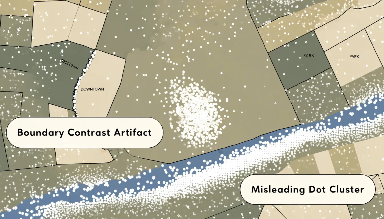
- Reading random dots as exact locations: When dots are distributed randomly within an enumeration unit like a census tract or ZIP code, a dot’s position is merely a visual placeholder for an aggregated quantity. Readers who treat these positions as exact addresses or buildings may draw false conclusions about proximity or clustering. For example, a cluster of dots near a park might suggest residents live inside it, when the dots are simply scattered across a larger tract that includes the park.
- Misreading boundary and border artifacts: Filling polygon areas with dots can create artificial visual edges where two enumeration units meet. If adjacent tracts have different population densities, the border between them may show a stark contrast or a sharp line of dots. Readers often mistake this contrast for a physical barrier, neighborhood boundary, or sudden change in land use, when it is actually an artifact of arbitrary administrative boundaries and the placement algorithm.
Population Distribution
Demographers use dot density maps to translate census counts into settlement patterns. A state with a population concentrated in a few metropolitan cores shows dense clusters against wide empty stretches, while dispersed rural settlement appears as an even scatter.
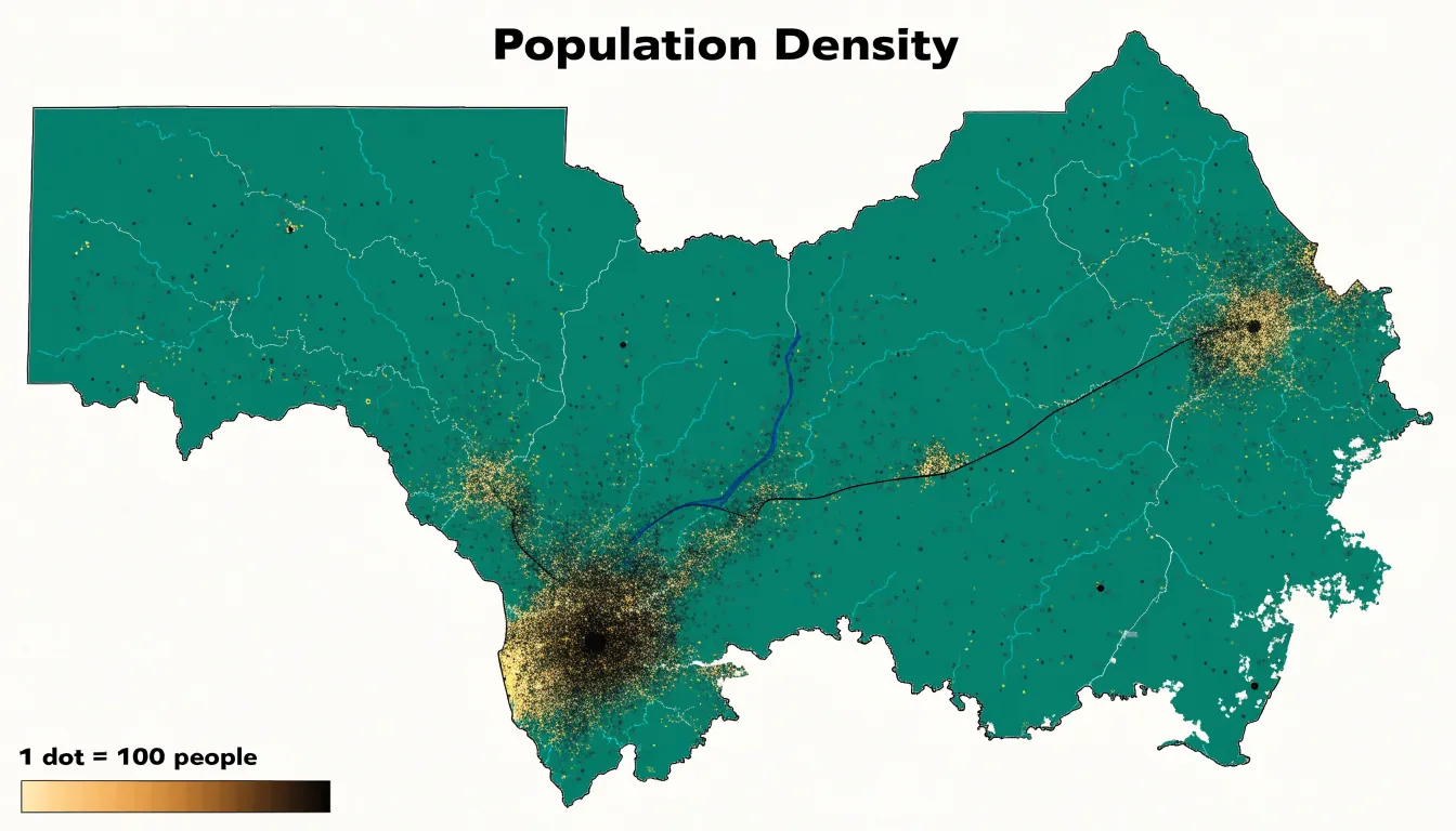
The workflow begins with census geography, where block-level counts are preferred because small units reduce placement distortion. Rather than scattering dots uniformly across a polygon, analysts often weight placement using ancillary data—such as land cover, road networks, or building footprints—toward developed land to avoid placing dots across uninhabitable terrain.
These maps support several applied demographic workflows:
- Urban planning: Visualizing sprawl and density gradients.
- Utilities and emergency services: Assessing how many residents fall within service areas.
- Public health: Overlaying population dots with environmental hazards to identify exposed populations.
- Election analysis: Comparing population distributions against voting district boundaries to evaluate representation.
Wildlife and Environmental Tracking
Ecologists and environmental scientists use dot density maps to track animal migrations, invasive species, and habitat shifts across landscapes and seasons.
- Animal migrations: Plotting radio-collar or citizen-science sightings as dots reveals migratory corridors, stopover sites, and range shifts over time, such as the gradual northward expansion of a species’ wintering grounds.
- Invasive species monitoring: Mapping confirmed sightings of an invasive plant or insect across successive years illustrates the speed and direction of spread. Resource managers use outlier dots to identify new introduction points for early detection and rapid response.
- Habitat shifts: Overlaying dot distributions with environmental variables like temperature or land cover correlates species occurrence with habitat alterations. For example, a denser cluster of dots along a shrinking wetland may indicate a population compressed into remaining suitable habitat. Time-series dot maps help quantify these range contractions or expansions for conservation planning and stakeholder communication.
Business Location Intelligence
Commercial analysts combine multiple dot density layers to guide site selection, targeted marketing, and resource allocation:
- Target demographics: Assigning dots to represent individuals with specific age, income, or lifestyle characteristics reveals fine-grained neighborhood concentrations within larger aggregate areas.
- Footprint density: Mapping existing customers or sales transactions as individual dots allows analysts to calculate kernel densities and pinpoint core customer zones. Comparing footprint density against demographic overlays separates proven markets (high footprint, strong demographics) from untapped potential (low footprint, favorable demographics).
- Competitor proximity: Plotting competitor locations as distinct dots alongside demographics and footprint data highlights underserved areas where demand exists but competition is sparse. Analysts also calculate drive-time polygons or distance bands around competitors to quantify trade areas and estimate reachable target customers.
- Composite opportunity index: By assigning weights to demographics, footprint, and competition based on business priorities, analysts generate heat maps that highlight areas with high demographic potential, low current penetration, and limited competition.
Choropleth vs. Dot Density
Choropleth maps shade entire regions—counties, census tracts, or ZIP codes—according to a summary statistic such as population density or category share. While effective for normalized rates and percentages that describe a region as a whole, choropleths struggle with raw counts and totals across regions of unequal size. Large rural polygons can dominate the map visually even when they contain very few people or events, a distortion known as regional area bias.
Choropleths are also vulnerable to the modifiable areal unit problem (MAUP): because administrative boundaries are arbitrary, changing the aggregation units (for example, from tracts to counties) can alter the apparent pattern without any change in the underlying data.
Dot density mapping mitigates both regional area bias and MAUP by pushing representation closer to individual observations, though random placement still relies on boundary containers. Use a dot density map when the data are discrete counts (such as disease incidents, farms, voters by party, or housing units), when spatial concentration matters more than regional averages, and when unequal polygon sizes would mislead. Reserve choropleth maps for normalized rates where the region itself is the unit of interest.
Data Preparation
Preparing spreadsheet data for a dot density map requires structuring, filtering, and normalizing the dataset before import:
- Review and structure attributes: Ensure each column represents a distinct variable and each row corresponds to a unique geographic observation (such as a census tract or city block) with its associated counts. Standardize headers, fix inconsistent naming conventions, remove stray spaces, and unmerge cells to prevent import errors.
- Filter records: Remove duplicate rows, address missing or incomplete entries, and exclude outliers that could skew the dot distribution. Filter out regions with zero counts if they would cause empty areas to map incorrectly.
- Normalize values: Where appropriate, convert raw counts into densities (such as people per square kilometer) or adjust for varying area sizes so the map reflects actual distribution rather than boundary artifacts.
- Verify geography: Check coordinate fields and confirm consistent geographic identifiers, such as FIPS codes, so records join cleanly to boundary files in mapping software.
Interactive and Mobile Mapping
Designing dot density maps for web and mobile platforms requires adapting to varying screen sizes, zoom levels, and touch interfaces:
- Responsive dot sizing: A dot pattern that reads clearly on a desktop monitor can become an indistinct smudge on a smartphone. Scale dot size proportionally with the display using relative units or dynamic sizing functions based on viewport dimensions.
- Adaptive aggregation: At low zoom levels on small screens, rendering every dot causes visual clutter and slows performance. Use a hierarchical data structure to cluster dots into larger symbols or density surfaces when zoomed out, transitioning to finer individual dots as the user zooms in.
- Touch-friendly interaction: Make interactive dot symbols large enough to tap accurately, and replace desktop hover interactions with tap or press events.
- Performance optimization: Limit rendered dots through viewport-based filtering and render via HTML5 Canvas or WebGL to keep panning and zooming smooth on resource-constrained mobile devices.
Ethical Mapping
Design decisions in dot density mapping shape how readers interpret real places and populations, carrying three main ethical responsibilities:
- Scale integrity: Adjusting the dot-to-value ratio can dramatize or erase perceived concentrations from identical data. Document the chosen ratio, apply it consistently across the map’s full extent, and test whether the visual pattern holds under reasonable alternative ratios.
- Placement transparency: Automated random-placement algorithms can inadvertently push symbols toward roads, waterways, or boundaries, fabricating apparent correlations with physical features. Check placement outputs against known geography, avoid algorithms that favor visually convenient locations, and disclose the placement method used.
- Spatial framing: Cropping a map to highlight a dense corridor while omitting surrounding emptiness tells a different story than showing the wider region. Include meaningful geographic context, choose an appropriate projection, state the dot value clearly in the legend, and add annotations that acknowledge uncertainty in the underlying counts.
Map Design Checklist
Before publication, review the dot density map against four design criteria:
- Legend clarity: State the unit value per dot, the mapped variable, and any scaling or aggregation rules. Place the legend where the eye travels naturally after the title, keep phrasing parallel across entries, and test it with an unfamiliar reader to ensure the map requires no verbal explanation.
- Accessible color palettes: Choose palettes that vary in lightness as well as hue rather than relying on red-green contrast alone. Run candidate colors through a colorblind simulator and verify that adjacent categories remain distinct at small sizes and low densities.
- Contrast ratios: Maintain legible contrast for text against backgrounds, dots against polygon fills, and legend swatches against labels on screen and in print. Avoid placing dots over busy basemap features that compete for attention.
- Visual hierarchy: Use size, weight, and spacing to guide the eye from the title to the legend, data layer, and footnotes. Reserve the strongest color and contrast for the dots so the data dominate the frame while source notes, scale bars, and annotations recede into a secondary tier. Check the finished map at thumbnail size to confirm the hierarchy holds up when reduced.
Frequently Asked Questions
What is a dot density map?
A dot density map places one dot for every fixed count of a phenomenon, spreading thousands of marks across a geographic area so the eye reads raw concentration directly. Dense clusters signal hot spots, while thinner areas show sparsity.
How do I choose the dot scale for a dot density map?
Start with the densest area the map must show, calculate how many dots that area would generate at a candidate scale, and check whether the symbols remain distinguishable. The busiest region should stay legible as a field of separate dots rather than a filled polygon, so test several values and compare the maps side by side.
What is the difference between exact and random dot placement?
Exact placement puts dots at precise geocoded coordinates, so the arrangement directly reflects the underlying data, but it requires highly granular data that is often unavailable or unreliable due to privacy concerns, incomplete records, or geocoding errors. Random distribution scatters dots within administrative polygons to preserve overall density while obscuring individual locations to protect confidentiality, though it can smooth out local variations.
How large should dots be on a dot density map?
The pixel radius determines how much ink lands on the canvas and how legible each mark stays. A radius that is too large makes neighboring dots overlap into solid blocks, while one that is too small leaves dots as isolated specks; test several radii against the densest area and select the largest value that still preserves visible white space between individual dots.
How is a dot density map different from a choropleth map?
Choropleth maps shade entire regions according to a summary statistic and work well for normalized rates and percentages, but they struggle with raw counts and totals across regions of unequal size, causing regional area bias. Dot density mapping mitigates regional area bias and the modifiable areal unit problem by pushing representation closer to individual observations, though random placement still relies on boundary containers.
What are common misreadings of dot density maps?
Readers often misread randomly distributed dots as exact locations, when a dot’s position is merely a visual placeholder for an aggregated quantity. They may also mistake border contrasts between adjacent enumeration units for physical barriers or sudden land-use changes, when these can be artifacts of arbitrary administrative boundaries and the placement algorithm.
Tony Astor
Tony writes about data visualization and the tools people use to build charts and dashboards. More about Data Illustrator