Density Plot: Visualizing a Distribution Smoothly
 By Tony Astor ·

Density Plot
A density plot is a smooth, continuous curve showing how values in a dataset are distributed, created by kernel density estimation, which sums small kernel bumps centered on each observation. The horizontal axis shows values, the vertical axis shows density, and the total area under the curve equals one, so areas correspond to probabilities.
Table of Contents
Density Plot
A density plot offers a smooth, continuous view of how values in a dataset are distributed. The easiest way to understand it is to start with a familiar picture: a histogram. A histogram sorts observations into bins and draws a bar for each bin, with the height reflecting how many observations fall inside. While effective, the result depends heavily on the number and width of the bins, and the stair-step outline can feel blocky. A density plot takes the same underlying data and replaces those bars with a flowing curve that traces the overall shape of the distribution.
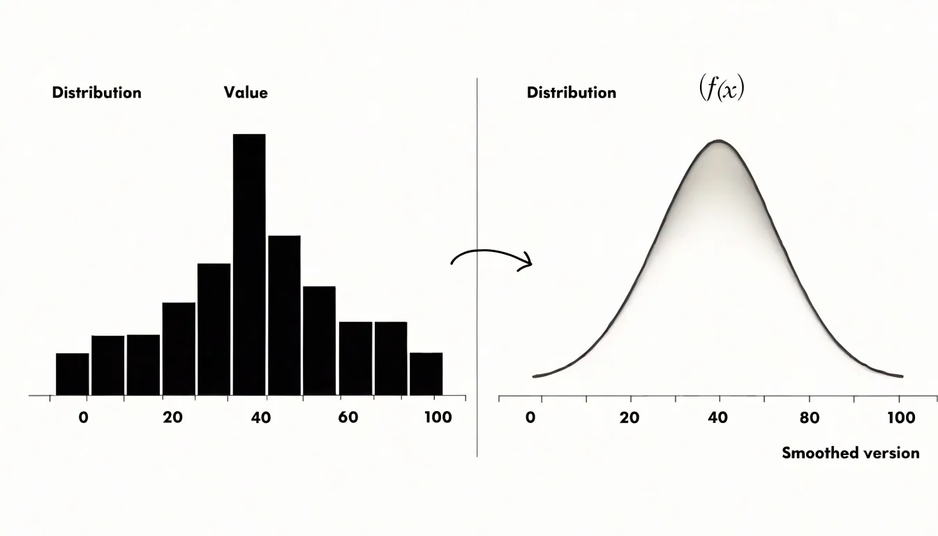
The transformation happens through a process called kernel smoothing. Each individual observation is treated as a small bump centered on its own value, and these bumps are added together across the whole dataset. Where observations cluster closely together, the bumps overlap and the curve rises; where observations are sparse, the curve stays low. The resulting shape communicates where values concentrate, how spread out they are, and whether the distribution is symmetric or skewed.
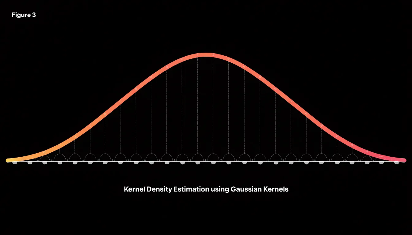
The horizontal axis shows the values of the variable itself, while the vertical axis represents density rather than raw counts. Beginners often find it helpful to think of the height of the curve at any point as indicating how likely values near that point are to occur. The total area under the curve equals one, which allows distributions of different sizes to be compared directly.
One practical consideration is the smoothing parameter, often called the bandwidth. Choosing an appropriate bandwidth is a balance between capturing local detail and revealing the broader pattern.
Density Plot vs Histogram
Histograms and density plots both visualize the distribution of continuous data, yet they introduce different analytical tradeoffs. Because a histogram counts observations in discrete bins, each bar corresponds to a concrete tally of data points. However, the visual result can shift noticeably when bin boundaries or starting positions are adjusted, and fine structure within a bin remains hidden. Density plots estimate a continuous probability density function without the blocky artifacts of binning, and small bandwidth changes affect smoothness rather than alignment.
Choosing between the two depends on the analytical goal and sample size:
- Histograms suit situations where exact counts matter, sample sizes are modest, or audiences benefit from a direct tally of observations.
- Density plots excel when the focus is the underlying shape of a continuous variable, when comparing several distributions on shared axes, or when a polished, continuous summary is desired.
Sample size also interacts with the choice. Sparse data can make kernel estimates look artificially smooth or produce spurious bumps near the edges, while large samples let both methods reveal subtle features, with density curves often making multimodality easier to spot.
Practical analysts frequently pair the approaches, using a histogram to ground the reader in raw counts and overlaying a density curve to communicate the smoothed trend. Bandwidth and bin width act as analogous tuning parameters; neither view is inherently more truthful, as each highlights some features and softens others.
Kernel Density
Kernel density estimation (KDE) builds a density curve by placing a symmetric shape—a kernel function, such as a Gaussian bell—centered on each observation’s value. The kernel determines how the observation’s influence spreads outward: near the center the contribution is large, and it tapers off with distance according to the chosen shape. When the individual kernels are summed at each location along the horizontal axis, the overlapping tails and peaks combine into a single continuous line.
Mathematically, the estimate at any point $x$ is the average of the kernel values evaluated at the distances between $x$ and every observation. In practice, this means sliding a window across the data range and accumulating contributions from nearby points, weighting closer observations more heavily. The height of each bump is scaled so that the total area under the combined curve equals one.
This additive summation explains why the curve is smooth even when the underlying data are sparse or unevenly spaced: the kernel shapes fill gaps and soften abrupt jumps. Regions with clustered observations receive many overlapping contributions and rise into peaks, while empty regions receive only the fading tails of distant kernels and settle into low valleys.
Bandwidth Selection
The bandwidth parameter, often denoted as $h$, controls the trade-off between smoothness and fidelity by determining the width of the kernel function placed at each data point.
A small bandwidth produces a narrow, tall kernel, causing the estimated density to closely follow individual data points. This leads to an under-smoothed plot where the curve appears jagged and noisy, reflecting random fluctuations that can obscure true patterns like modes or skewness.
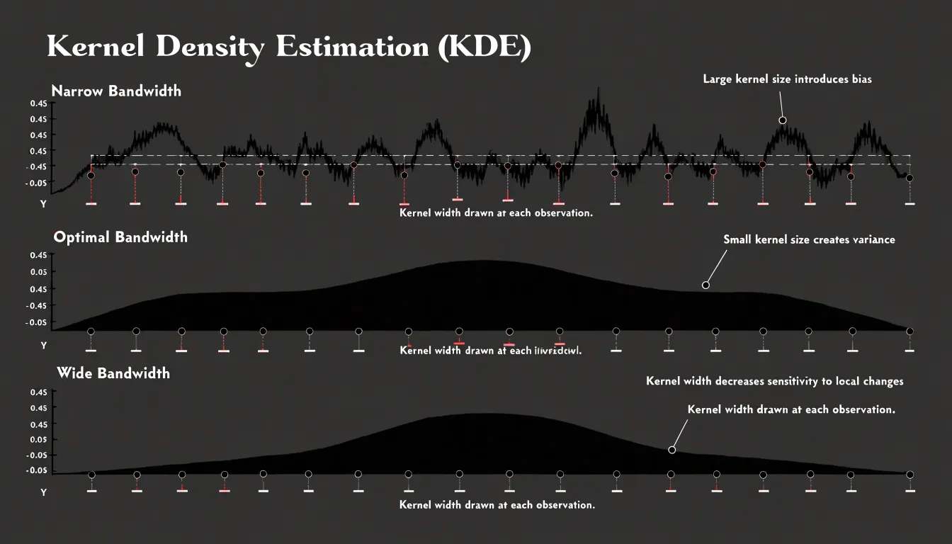
Conversely, a large bandwidth results in a wide, short kernel that averages over a larger neighborhood of points. This produces an over-smoothed, flattened plot where important details may be hidden. For instance, a bimodal distribution might appear as a single broad hump, leading to incorrect conclusions.
Statistical methods, such as cross-validation or plug-in estimators, aim to minimize the mean integrated squared error, providing an optimal bandwidth that captures essential structure without overfitting to noise. In practice, the choice also depends on sample size. With large datasets, a smaller bandwidth can be used without introducing excessive noise, while small datasets may require a larger bandwidth to avoid spurious artifacts.
Shape Reading
Reading a density curve starts with scanning for the peak—the point where the curve reaches its highest value—which indicates where the typical case sits on the horizontal axis. When a curve shows two distinct peaks separated by a dip, the data likely contains two subgroups clustering around their own centers. Counting peaks is a fast way to detect latent groups before running formal clustering analysis.
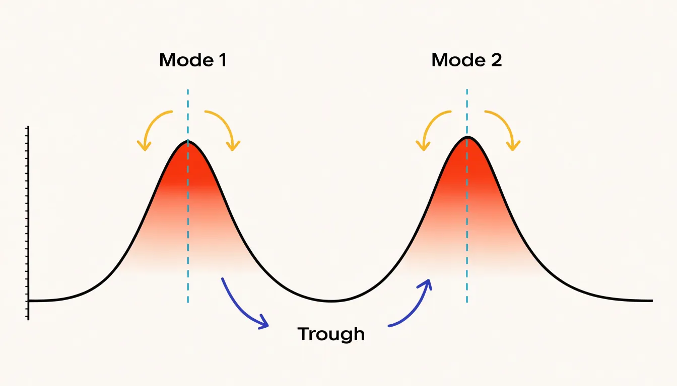
Troughs carry equal diagnostic weight. A deep valley between two modes signals a genuine separation between groups, while a shallow dip suggests the groups overlap and blend into one another. The width and height of the valley give a rough sense of how distinct the subpopulations are.
Spread is the next feature to assess. A narrow, tall curve means values cluster tightly around the center, while a wide, flat curve means values scatter broadly. Comparing spread across multiple curves on the same axis makes differences in variability immediately visible.
Finally, inspect the tails. Asymmetry in the curve—where a long tail stretches to one side—indicates skewness and points to extreme values. Isolated bumps far from the main mass often represent small groups of unusual observations or outliers. Starting at the peak and sweeping outward along both slopes yields a working hypothesis about center, grouping, and variability before any summary statistics are computed.
Area Under the Curve
Because a density curve is normalized so that the total area beneath it equals one, the curve represents a complete distribution of outcomes for a continuous random variable. Analysts rely on this normalization to translate geometry into meaning: area becomes probability.
When a sub-region of the curve is shaded, its area corresponds to the estimated probability that a randomly drawn observation falls within that interval. For example, the area under the curve between 20 and 30 gives the probability that an observation lands inside that range. A wider interval captures more area and a higher probability, while a narrow interval captures less. Because the total area equals one, each sub-region falls between zero and one, and probabilities across non-overlapping intervals sum consistently.
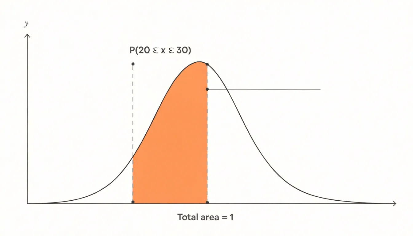
Rather than working with raw counts, analysts can compare regions directly to ask how likely a value is to exceed a threshold, or how much probability mass sits in a particular band. This correspondence also clarifies why the height of a density curve is not itself a probability; height reflects concentration, while accumulated area carries the probabilistic interpretation.
Group Comparison
Overlaying multiple density curves on a single plot compares distributions across categorical groups, revealing differences in shape, central tendency, spread, and multimodality that might be obscured in separate side-by-side plots. Each group’s density estimate is computed separately and layered onto the same axes. The primary design challenge is keeping all curves visible where they overlap.
Common approaches to managing overlap include:
- Transparency (alpha blending): Setting a low alpha value (e.g., 0.3 to 0.5) for the fill color makes overlapping regions darker, indicating where distributions coincide. This works well for two or three groups, though more groups can make the plot cluttered and the colors muddy.
- Ordered solid fills: Distinct colors with solid fills can be used if plotted in a specific order (e.g., from largest to smallest area) so smaller distributions are not completely hidden.
- Outlines: Using outlined curves without fill avoids occlusion but can make the overall shape harder to perceive. Combining a transparent fill with a solid outline often strikes the best balance.
For accurate comparisons, use a consistent bandwidth across all groups, as differing smoothing parameters can distort shapes. Always include a legend or direct labels to identify each group. When comparing many groups, small multiples (separate panels) or ridge plots are often more effective than a single overlaid chart.
Skewness Detection
Skewness detection focuses on the tails stretching away from the central mass of the distribution:
- Positively skewed: The right-hand tail extends further and thins out more gradually than the left side, indicating that a small number of unusually large values are pulling the mean upward.
- Negatively skewed: The left tail stretches out toward smaller values, while the bulk of the observations sit toward the higher end of the range.
Spotting these extended tails reveals patterns that summary statistics conceal, whether you are examining incomes, response times, or measurement errors. Two datasets can share an identical mean and standard deviation while having radically different shapes, so a report built only on those numbers may suggest symmetry where none exists. A density plot exposes whether the central peak is offset, whether one shoulder is heavier, and whether extreme values cluster in a way the average cannot communicate.
Simple tail inspection can still miss hidden skew patterns. Bimodal distributions, mixtures of subpopulations, or data with a hard boundary can produce apparently symmetric overall shapes while concealing lopsided behavior within subgroups. Overlaying density curves for different categories or zooming in on the tails helps uncover these subtler departures. Comparing the positions of the mean, median, and mode provides a useful numerical cross-check, since skewness shifts these measures apart in predictable directions.
Bimodal Data
Bimodal data exhibits two distinct local peaks (modes) rather than a single central peak, signaling hidden heterogeneity or a mixture of sources within a dataset. For example, customer ages from a retail store might peak around young adults and again around older adults, reflecting two distinct shopping demographics. Similarly, measurements of a physical process might show two peaks if two machines produce the same part with slightly different settings. Bimodality can also arise from data errors or mixed measurement scales, making peak detection a useful data quality check.
Ignoring bimodality leads to misleading summary statistics: the mean of a bimodal distribution may fall right in the valley where few observations exist, and the overall standard deviation may be artificially inflated. Once a density plot makes the two peaks apparent, analysts can separate the data into subgroups, incorporate a categorical variable that explains the split, or choose more appropriate segmentation strategies.
Sample Size and Outliers
A density plot’s reliability depends heavily on sample size. With a large sample, the estimated curve tends to be stable. When the sample is small, each observation carries considerable weight, and the smoothing process has little information to work with. A sample of a dozen points may produce multiple humps simply because the bandwidth interacts awkwardly with the sparse spacing of observations, and adding a few more points can change the shape dramatically. Treat density estimates from small samples with caution, as apparent structure may be an artifact of random variation.
Extreme values exert a similarly strong influence, particularly on the tails. An outlier sitting far from the main body of data stretches the horizontal axis and forces the kernel to place density in an otherwise empty region, producing a long, thin tail or a small secondary bump that exaggerates the importance of a single point. Because the total area under the curve is fixed at one, spreading density outward into the tails necessarily lowers the height of the curve elsewhere, flattening the central peak and making the main cluster appear less concentrated than it truly is. Analysts should inspect data for extreme values before interpreting a density plot, considering robust smoothing methods or explicit outlier handling so the curve reflects the bulk of the data.
Two-Dimensional Density Plots
A two-dimensional density plot extends one-dimensional KDE into a plane, placing two continuous variables on the horizontal and vertical axes and representing the local concentration of observations as a continuous surface. Rather than showing how a single variable is distributed, it maps the joint probability distribution—showing where pairs of values cluster together and revealing the shape, spread, and orientation of the relationship between the two variables.
With large samples, where a standard scatter plot collapses into an unreadable cloud of overlapping points, a smoothed 2D density surface preserves interpretable structure. The surface can be rendered in several ways:
- Filled color gradients: Assign lighter or darker shades to regions of high and low density, giving an immediate impression of where the mass of the data lies.
- Contour lines: Drawn at fixed density thresholds, these work like elevation lines on a topographic map to trace the boundaries of concentrations.
- Combined shading and contours: Color conveys magnitude while lines emphasize structure.
Contour shapes reveal specific bivariate features: concentrated rings or ellipses indicate a strong central tendency, elongated bands suggest correlation between the variables, and multiple separate islands of high density point to distinct subgroups or multimodal behavior. Outliers appear in sparse regions far from the main contours.
Combining Charts
Layering a density curve with a boxplot combines complementary strengths into a single hybrid view. A boxplot provides a compact five-number summary—minimum, first quartile, median, third quartile, and maximum (or whisker endpoints)—while flagging outliers as individual points beyond the whiskers. However, reducing the data to these summary statistics conceals multimodality or gaps. Adding a density curve restores the full distributional shape alongside the exact quartiles.
A popular implementation of this combination is the raincloud plot, which places a half-density curve (the “cloud”) above or beside a boxplot, paired with a jittered strip of individual data points (the “rain”) below it. This layout is especially effective for group comparisons, allowing viewers to compare medians and quartiles while simultaneously seeing raw sample sizes and distributional shapes. When building hybrid plots, ensure that the scales align and position the density curve so it does not obscure the boxplot elements.
Real-World Applications
Across industries, density plots serve as diagnostic tools for inspecting large volumes of continuous measurements:
- Finance: Banks plot transaction amounts across a customer base to see where normal activity sits versus thin tails of large transfers, informing fraud thresholds. Credit teams compare repayment delay densities across customer segments, and trading desks examine daily return distributions to gauge volatility and the likelihood of extreme moves.
- Healthcare: Hospitals chart patient wait times, blood pressure readings, or laboratory values to spot clustering around abnormal ranges. Public health analysts overlay densities from different regions or time periods to evaluate whether an intervention shifted typical values, and clinicians examine group overlap to judge how well a screening threshold separates healthy patients from those needing follow-up.
- Technology: Engineering teams visualize request latency, CPU utilization, or error rates to see whether most responses are fast while a small fraction drags into slow territory. Product managers plot session durations or feature usage to identify engagement peaks that suggest distinct user habits.
Common Mistakes
Because density plots look smooth and authoritative, their polish can hide design choices that distort the underlying data:
- Truncating the horizontal axis: Cutting the axis tightly at the smallest and largest observed values clips the tails of the distribution and makes the curve appear to drop abruptly to zero, suggesting a sharp boundary that does not exist. Extend the axis slightly beyond the data range so viewers can see how the distribution naturally tapers.
- Relying on a single arbitrary bandwidth: Setting the bandwidth too wide dissolves secondary peaks or shoulders into a single hump; setting it too narrow turns random noise into spurious spikes. Test several bandwidths to see how the curve responds—a finding that survives smoothing changes is far more trustworthy than one that appears at a single setting.
- Over-interpreting sparse regions: Where observations are scarce, the kernel estimator spreads individual points into gentle bumps that reflect sampling noise rather than real structure. Building narratives around small tail bumps misleads readers who cannot see how few points support that part of the curve. Adding a rug plot or histogram underneath the curve makes sample density visible and tempers overconfidence.
Overview
Several mature libraries generate density plots directly:
- Python: Seaborn’s
kdeplothandles statistical computation and rendering in a single call,pandasexposes a density option through its plotting interface, andmatplotlibprovides low-level control for custom styling. - R:
ggplot2builds density plots viageom_density, supporting layering, faceting, and extensions within the grammar of graphics.
When styling a plot for production, label both axes clearly (including units for the horizontal variable) and use annotations to call out key modes or thresholds. A filled area with modest transparency often reads more clearly than a bare line. For deeper study and worked examples, consult the official documentation for Seaborn and ggplot2, the R Graphics Cookbook, textbooks on statistical graphics, and reproducible notebooks on public repositories.
In an ongoing analytics workflow, wrapping density plot code into reusable functions and regenerating charts alongside summary statistics when data refreshes helps surface distribution shifts that aggregate tables miss.
Frequently Asked Questions
What is a density plot?
A density plot is a smooth, continuous view of how values in a dataset are distributed, created by replacing histogram bars with a flowing curve through kernel smoothing.
What does bandwidth do in a density plot?
The bandwidth controls the trade-off between smoothness and fidelity by setting the width of the kernel placed at each data point. A small bandwidth can produce an under-smoothed, jagged curve, while a large bandwidth can over-smooth and hide details such as a second mode.
When should I use a density plot instead of a histogram?
Histograms suit exact counts, modest sample sizes, or audiences needing a direct tally, while density plots excel when the focus is the underlying shape of a continuous variable, comparing several distributions, or a polished continuous summary.
How do you read the shape of a density plot?
Scan for peaks to find typical cases or possible subgroups, check troughs to judge how distinct groups are, and assess spread and tails for variability, skewness, and outliers. A narrow, tall curve means values cluster tightly, while a wide, flat curve means values scatter broadly.
What does the area under a density curve represent?
Because a density curve is normalized so the total area equals one, the area under a sub-region corresponds to the estimated probability that an observation falls within that interval. The height itself is not a probability; height reflects concentration, while accumulated area carries the probabilistic interpretation.
Are density plots reliable with small samples or outliers?
Treat density estimates from small samples with caution, because sparse data can produce humps that change dramatically with a few more points and may be artifacts of random variation. Extreme values can also stretch the horizontal axis, create long tails or small secondary bumps, and flatten the central peak, so analysts should inspect for extreme values before interpreting the plot.
Tony Astor
Tony writes about data visualization and the tools people use to build charts and dashboards. More about Data Illustrator