Dendrogram: How to Read a Hierarchical Clustering Tree
 By Tony Astor ·

Dendrogram
A dendrogram is a branching tree diagram that visualizes hierarchical relationships among items, where merge heights on the vertical axis represent the distance or dissimilarity between clusters—short branches mean items are very similar, tall branches mean they are quite different. It is produced by hierarchical clustering of a pairwise distance matrix.
Table of Contents
Dendrogram Basics
A dendrogram is a branching diagram that visualizes the hierarchical relationships among a set of items. The vertical axis typically represents the distance or dissimilarity between clusters, with lower values indicating greater similarity. The horizontal axis lists the individual data points, often arranged so that similar items are placed close together. When two items or clusters merge, their branches join at a height corresponding to the distance between them. This height is a direct measure of how dissimilar the merged groups are: short branches mean the items are very alike, while tall branches indicate that the groups are quite different.
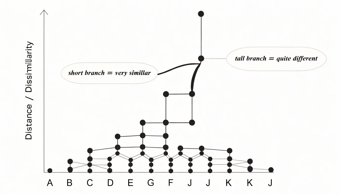
By reading the tree from bottom to top, you can trace the sequence of merges and see how individual constituents gradually combine into larger clusters. The pattern of branching reveals the overall structure of the data, highlighting which items are most closely related and which are more distinct. Interpreting a dendrogram requires attention to the scale of the vertical axis, as the absolute distances matter for understanding the degree of similarity. The horizontal axis order is often optimized to reduce crossings, but it does not affect the underlying clustering.
Hierarchical Clustering
Hierarchical clustering is the method that transforms a shelf of individual essential oils into an organized map of related groups. The process begins with each oil treated as its own separate item, defined by a set of measurable characteristics. These characteristics can include aromatic notes such as citrus, floral, or woody, along with chemical markers like the presence of linalool, limonene, or eugenol. Each oil becomes a point in this multidimensional space, and the distance between any two points reflects how similar their profiles are. Oils with closely matching aromas and chemistry sit near one another, while oils with little in common sit far apart.
The first step calculates similarity between every possible pair of oils using a distance measure, where small values indicate strong resemblance. Once all pairwise similarities are known, the algorithm identifies the two closest oils and merges them into a single cluster. This new cluster then takes on a representative profile, often the average of its members, and the similarity calculations are repeated with the cluster treated as a new item.
The merging continues in rounds. At each round, the closest pair of items, whether single oils or existing clusters, is joined to form a larger group. Early merges tend to pair oils with nearly identical profiles, such as two bright citrus oils. As the process advances, these small groups combine into broader categories, so that citrus clusters may join with other light, top-note oils, while resinous and woody oils gather separately. The order of merges records the entire hierarchy of relationships. Reading the resulting tree from the tips to the root reveals how individual oils gradually assemble into families, giving a clear picture of which oils share aromatic and chemical ground.
Bottom-Up and Top-Down
Hierarchical clustering proceeds by one of two directional strategies, and the choice shapes nearly every downstream property of the resulting dendrogram. The agglomerative, or bottom-up, approach begins with every observation occupying its own singleton cluster. At each step the algorithm merges the pair of clusters that are closest under a chosen linkage criterion, whether single linkage (nearest neighbors), complete linkage (farthest neighbors), average linkage, or Ward’s minimum-variance method. The process repeats until all observations fall within a single root cluster. The divisive, or top-down, approach reverses this logic: it starts with the entire dataset as one cluster and recursively splits it, typically by identifying the partition that maximizes between-group separation or minimizes within-group variance.
The computational asymmetry between the two is substantial. Agglomerative clustering requires on the order of n squared pairwise distance computations and is straightforward to implement, with the merge history yielding the dendrogram directly. Divisive methods must consider an enormous number of possible splits at the top levels; exhaustive search is infeasible for all but small samples, so practical implementations rely on heuristics such as recursive k-means bisection, and even then the procedure is costlier and more sensitive to early partitioning errors, since a poor first split cannot be repaired later.
For botanical data these properties matter concretely. Herbarium and survey datasets frequently involve hundreds or thousands of specimens described by morphological characters, and agglomerative clustering handles that scale comfortably while producing the nested, distance-scaled groupings taxonomists expect. Bottom-up merging also accommodates the incremental nature of botanical collections, where new specimens arrive over time and can be appended and re-clustered without rebuilding the entire hierarchy from scratch.
Branches and Lines
In a dendrogram, every branch and connecting line carries quantitative meaning. In horizontally oriented layouts, the horizontal axis represents the similarity or distance score, and the point at which two branches merge marks the exact level of similarity at which two samples or clusters are joined. The length of the line spanning from a merge point down to its child nodes therefore illustrates a specific score: a long branch corresponds to a large distance value, while a short branch corresponds to a small one. The position of merge points records the sequence in which similarity thresholds are crossed, moving from the finest distinctions at the tips of the tree toward broader groupings nearer the root, where the final merges reflect the most general relationships in the dataset.
When two oils share a very short connecting line, their profiles sit close together in the underlying similarity space, which signifies high chemical overlap between them. Such oils likely share dominant constituents, comparable ratios of major compounds, or closely matching profiles across the measured variables. The brief line tells the reader that little dissimilarity separates the pair and that distinguishing them would require finer measurement or a different analytical lens. Longer lines, by contrast, indicate that the clusters involved differ more substantially in composition. By scanning the lengths throughout the diagram, an analyst can quickly identify tightly knit groups of chemically similar oils and recognize the branches that bridge more distant families, supporting decisions about substitution, blending, sourcing, or quality control.
Height and Cutoff
The merge height on the distance axis is the primary tool for deciding where the tree should be split. Drawing a horizontal threshold line across the diagram at a chosen height partitions the blends into distinct groups: every branch intersected by the line belongs to a separate category, while branches that join below the line remain together in the same group. In practice, the analyst examines the sequence of merge heights from the bottom of the tree upward. A cutoff placed just below a large jump in merge height captures the natural break in the data and yields categories that reflect genuine differences among the blends.
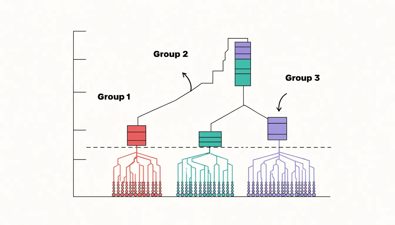
Selecting the height therefore involves a mix of quantitative guidance and practical judgment. One common approach is to inspect the gap between successive merge levels and place the line in the widest gap, since that gap signals the point at which distinct functional groups separate from one another. Another approach is to fix the number of desired categories in advance, based on how the blends will be used in formulation or marketing, and then set the height that produces exactly that number of branches. Both methods benefit from comparing several candidate cutoffs side by side. A lower cutoff produces many small, tightly defined groups, each with a narrow aromatic or therapeutic character; a higher cutoff produces fewer, broader groups that combine related blends under a single functional heading. Recording the blend composition of each resulting group alongside the chosen height makes the classification reproducible and allows the threshold to be adjusted later as new blends are added to the dataset.
Cladograms vs Dendrograms
Cladograms and dendrograms both take the form of branching trees, yet they encode different kinds of information and follow different rules of construction. A cladogram is a diagram of evolutionary relationships built from shared derived characters. Each branching point represents a hypothetical common ancestor, and each tip represents a taxon whose placement reflects descent from that ancestor. The branch lengths in a cladogram carry no quantitative meaning; they are drawn for legibility, and the topology alone conveys the hypothesis. A dendrogram, by contrast, is a general-purpose tree produced by hierarchical clustering of a distance or similarity matrix, with branches scaled to the measured distance between clusters. Nothing in the algorithm requires that the distance reflect genealogical descent; the same procedure clusters chemical spectra, gene expression profiles, or survey responses with equal ease.
In a cladogram, the data are discrete character states scored across taxa and analyzed with parsimony, likelihood, or Bayesian methods, and the resulting tree is a claim about history. In a dendrogram, the data are pairwise distances, and the tree is a summary of similarity that depends on the clustering algorithm, the linkage rule, and the distance measure selected. Those choices can reshuffle the topology even when the underlying distances are unchanged.
The practical consequence is that a dendrogram built from chemical affinity among samples can look exactly like a phylogeny while meaning something entirely different. Two specimens may cluster together because they share a compound profile, a solvent system, or a sampling site, and that proximity says nothing about shared ancestry. Readers who treat such a diagram as an evolutionary tree risk reading genetic relationship into what is only chemical resemblance. Identifying which kind of tree is on the page begins with the axis labels and the methods described in the caption, and it determines how much historical weight the branches can bear.
Distance Measures
Every dendrogram begins with a matrix of pairwise distances, and the choice of distance measure shapes everything that follows. Distance measures translate the raw data for each extract into a single number that expresses how dissimilar two samples are, and the mathematical form of that translation determines which kinds of variation the clustering will notice.
Euclidean distance is the most familiar metric. It treats each variable as a coordinate in a multidimensional space and computes the straight-line separation between two points, taking the square root of the sum of squared differences across all variables. A difference of five percentage points on one constituent contributes twenty-five to the squared sum, while a difference of two contributes four. This squaring gives Euclidean distance a sensitivity to large deviations: samples that diverge strongly on even a single constituent register as far apart, which suits analyses where pronounced differences should dominate the similarity picture.
Manhattan distance takes a different route. Instead of squaring, it sums the absolute differences along each dimension, effectively measuring distance travelled along a grid rather than through open space. Because no term is squared, each percentage-point variation contributes in direct proportion to its size, and no single constituent can overwhelm the total. This makes Manhattan distance more robust when the data contain outliers or when many small, consistent differences together carry meaningful information about composition.
Both metrics operate on the constituent percentages directly, so the scale and number of variables matter. Analysts often standardise or weight the variables beforehand so that a constituent measured on a larger range does not swamp the others. The resulting distance matrix feeds the next stage of the procedure, where linkage rules decide how clusters merge. Selecting Euclidean or Manhattan distance is therefore an interpretive decision as much as a computational one, encoding assumptions about which percentage variations between extracts ought to count most heavily when similarity is judged.
Linkage Methods
Linkage criteria determine how the distance between two clusters is measured when a dendrogram is being built, and the choice among single, complete, and average linkage has a direct effect on the shape and structure of the resulting tree. Single linkage defines the distance between two clusters as the distance between their closest pair of members. Because it only needs one nearby pair to justify a merge, single linkage tends to chain clusters together through intermediate points, producing long, elongated branches and trees that can stretch across the data space. This chaining behavior makes single linkage sensitive to noise and often yields a topology with a few sprawling clusters rather than compact, well-separated groups.
Complete linkage takes the opposite extreme and measures cluster distance by the farthest pair of members. A merge occurs only when every point in one cluster is reasonably close to every point in the other, which encourages compact, roughly spherical clusters of similar diameter. In the dendrogram, complete linkage typically produces more balanced branching with shorter, tighter branches, and it resists the chaining effect that characterizes single linkage. The trade-off is that outliers within a cluster can inflate the distance and delay otherwise sensible merges.
Average linkage occupies a middle position, defining cluster distance as the mean distance over all cross-cluster pairs. This averaging smooths out the influence of individual extreme points, so the resulting topology tends to fall between the elongated chains of single linkage and the compact balls of complete linkage. Average linkage often produces trees with moderately balanced structure and is less sensitive to single outliers than complete linkage while avoiding the chaining problem of single linkage. Across all three methods, the same underlying proximity data can generate visibly different dendrograms, with branch lengths, merge heights, and cluster boundaries shifting according to which criterion governs the distance calculation.
Real-World Example
A concrete way to see a dendrogram at work is to cluster a small collection of essential oils by their dominant chemical constituents. Suppose we have six oils, including lavender, clary sage, bergamot, peppermint, eucalyptus, and tea tree. For each oil we record the relative percentages of two important compound families: monoterpenols, such as linalool and geraniol, and esters, such as linalyl acetate. These two variables give every oil a simple coordinate pair, which makes the underlying mathematics easy to follow while still reflecting real chemotypic distinctions that aromatherapists and formulators care about.
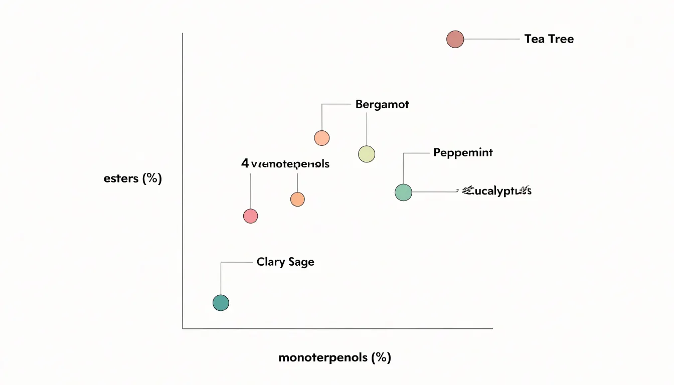
We begin by calculating the distance between each pair of oils, typically using Euclidean distance on the standardized percentages. Lavender and clary sage both show high concentrations of linalyl acetate and linalool, so their points sit close together and their pairwise distance is small. Bergamot, which is rich in linalyl acetate but lower in linalool, lands nearby but slightly farther out. Peppermint and eucalyptus, dominated by monoterpenols and oxides with very little ester content, cluster on the opposite side of the space. Tea tree, with its high terpinen-4-ol share and minimal esters, forms its own distinct position.
The clustering algorithm then merges the closest pair first, joining lavender and clary sage into a single branch. It recomputes distances between this new cluster and the remaining oils, often using average linkage, and continues merging step by step. Bergamot joins the lavender-clary sage branch next because its ester profile resembles theirs. Peppermint and eucalyptus pair up on the monoterpenol-heavy side, and tea tree attaches last, reflecting its unique chemistry.
Reading the finished dendrogram from left to right, the height of each horizontal join indicates how dissimilar the merged groups were. A formulator can use these branches to substitute oils within a cluster, while a quality chemist can spot samples that fall outside their expected branch.
Common Mistakes
One of the most persistent sources of confusion when working with dendrograms is the meaning of the horizontal axis. In a standard vertical dendrogram, every leaf sits along the baseline, with branches extending upward and connecting horizontally at the nodes where clusters merge. Because the horizontal bars stretch across the page at varying lengths, it is tempting to treat the lateral span of a branch as a measure of similarity or distance between items. This reading is almost always mistaken. The horizontal placement of a leaf carries no quantitative meaning at all; the drawing simply spreads the items out for legibility, and the order of nodes along the horizontal axis is an arbitrary convention chosen by the plotting software. Two items sitting side by side near the left edge are not necessarily more similar than two items placed far apart, and a long horizontal bar does not indicate a large distance.
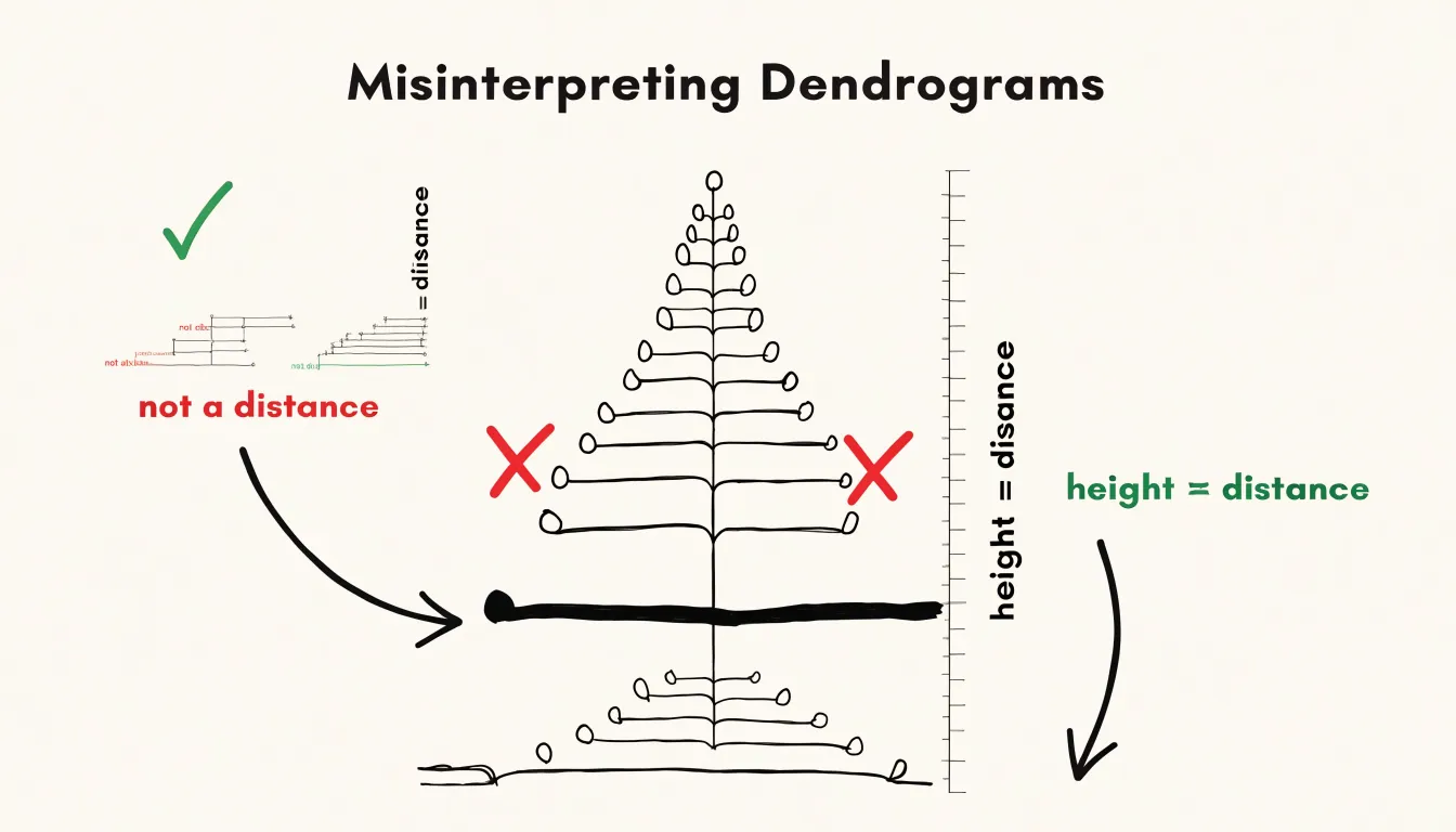
The quantity that matters is the y-coordinate of a node along the vertical axis. When comparing two merges, the correct comparison is between their heights, not between the lengths of the horizontal segments that lead to them. A common error is to glance at a wide, sprawling branch and conclude that its members are distant from one another, when in fact the relevant information is the vertical position of the junction joining them.
Readers should also be wary of inferring absolute distances from height alone without knowing the linkage method, since different clustering algorithms assign heights differently. Interpreting the dendrogram as a precise map of pairwise distances, rather than as a hierarchical ordering with merge heights, invites false conclusions about how closely related the underlying observations really are.
Heatmap Combinations
A heatmap combination pairs a dendrogram with a colored matrix whose rows or columns correspond to the leaves of the tree. The dendrogram supplies the ordering and the grouping, while the matrix carries the measured values, so that each variable’s behavior can be read in step with the cluster structure. In the layout most often used, the dendrogram occupies a margin along one side and the matrix fills the main field, with cells shaded according to the magnitude of the underlying value. Because the matrix rows are reordered to match the leaf order of the tree, similar samples sit next to one another and similar variables stack into contiguous bands. The eye can then follow a branch down into the rows it contains and see, at a glance, which columns brighten or darken together.
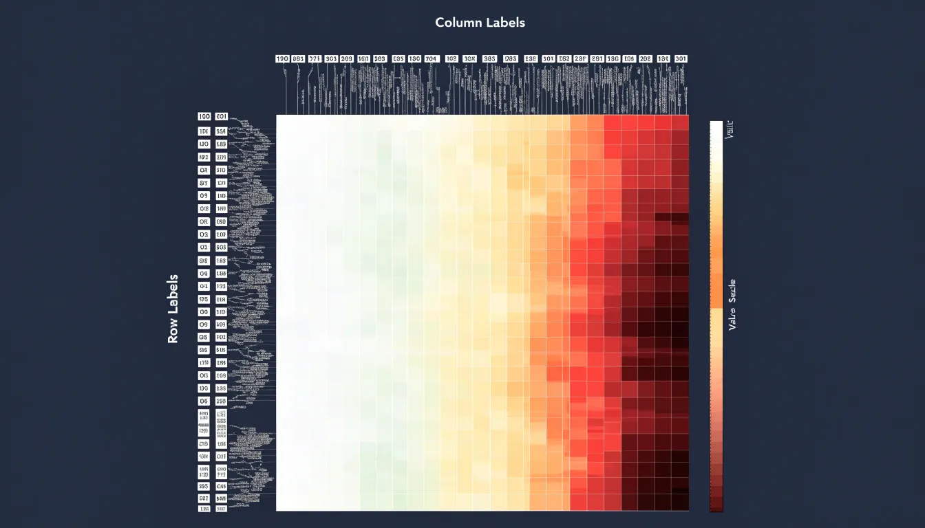
In blend formulation, the matrix columns can hold the concentrations of individual constituents while the tree summarizes the overall similarity of oil samples or candidate mixtures. A formulator reading the combined display sees where a grouping is driven by a dominant component and where differences arise from several minor constituents at once. The tree answers which blends belong together; the colored cells answer why, pointing to the specific constituents whose proportions shift between groups. This side-by-side presentation reduces the guesswork of cross-referencing a cluster list against a separate table of measurements, since the evidence sits directly beneath the branch it explains.
Such combined views also make outliers and transitional cases easier to place. A sample that joins a cluster late in the tree often shows a cell pattern intermediate between two color regimes, revealing it as a borderline blend rather than a clean member. Repeated examination of these patterns supports the intuitive formulation work of tuning proportions toward a target group, and the figure can serve as a shared reference when the reasoning behind a proposed blend needs to be communicated to others.
Software Tools
A range of software tools exists for generating dendrograms from chemical profile data, catering to different levels of technical expertise and use cases. For researchers and analysts who prefer a point-and-click interface, web-based applications offer an accessible entry point. These platforms typically allow users to upload a spreadsheet of chemical measurements, select a distance metric and linkage method, and produce a custom dendrogram without writing code. Many include interactive features such as zooming, node collapsing, and color-coding to highlight clusters, making them suitable for exploratory analysis and presentation.
For those working in programming environments, data packages provide greater flexibility and reproducibility. In R, packages such as dendextend and factoextra extend the functionality of base hclust and heatmap.2, enabling fine-tuned control over tree appearance, cluster labeling, and integration with other statistical workflows. Python users can leverage scipy.cluster.hierarchy and seaborn to generate dendrograms alongside heatmaps, while libraries like plotly and bokeh support interactive visualizations. These packages are particularly valuable when chemical profiles are large or when dendrograms must be embedded in automated pipelines.
Dedicated cheminformatics tools also exist, offering specialized functions for handling molecular fingerprints and similarity matrices. Commercial software such as MATLAB and JMP include clustering and dendrogram capabilities within broader statistical environments, often with graphical user interfaces that appeal to industrial users. Open-source alternatives like Orange and KNIME provide visual programming interfaces where users can build workflows by connecting data preprocessing, clustering, and visualization nodes.
When selecting a tool, considerations include the size of the dataset, the need for customization, the availability of support for specific distance metrics, and the desired output format. Documentation and community forums further influence usability, as does compatibility with existing data analysis ecosystems.
Practical Benefits
Formulators can read a dendrogram’s map of chemical kinship directly when composing custom botanical blends. When two botanicals sit close together on the chart, they share much of their marker compounds, essential oil constituents, or phytochemical fingerprints, which makes them plausible candidates for substitution. A formulator facing a supply shortage of one herb can scan the nearby branches and identify alternatives whose profiles overlap enough to preserve the intended character of the blend. The same logic supports deliberate blending: ingredients drawn from different regions of the dendrogram bring complementary constituents, so a recipe can be assembled to cover a broader spectrum of actives rather than stacking redundant ones.
Proximity analysis also helps balance a formula. If several chosen botanicals cluster tightly, the blend may concentrate similar compounds and leave gaps elsewhere, a pattern the dendrogram makes obvious at a glance. Formulators can then reach across the tree for ingredients from distant clusters to round out the profile. Distance values on the branches offer a rough guide to how much displacement a substitution introduces, letting a formulator decide whether a close neighbor will pass unnoticed or whether a farther branch will noticeably alter the mix. Documenting these choices against the dendrogram also creates a record that others can follow, so reformulation becomes a traceable step rather than a guess. Over repeated projects, the chart becomes a working reference, shortening the search for compatible ingredients and reducing the trial-and-error cycle that otherwise consumes time and material in the development of new botanical blends.
Quick Reference
When you first encounter a dendrogram in essential oil research, a systematic approach helps you extract meaningful information quickly:
- Check the axes: Examine the vertical axis to understand the distance or dissimilarity measure used, then identify the horizontal axis labels, which may be coded (e.g., sample IDs) or descriptive (e.g., plant species and origin).
- Trace the top-level splits: Look for the highest nodes first, as they define the major groupings in your data. Trace down from these splits to see which samples belong to each major branch.
- Count the clusters: Identify a large gap in merge heights—a point where the distance jumps significantly—and count the number of branches below that gap to decide how many clusters to retain.
- Examine cluster composition and outliers: Check whether samples are grouped by species, geographical origin, or chemical profile to interpret their biological or practical meaning. Note any outliers that merge at very high distances or form isolated branches, as these may warrant further investigation.
- Verify the methods: Note the linkage method (e.g., complete, average, Ward’s) and distance metric (e.g., Euclidean, Manhattan), as these choices affect the tree’s shape.
Frequently Asked Questions
What is a dendrogram?
A dendrogram is a branching diagram that visualizes the hierarchical relationships among a set of items. The vertical axis typically represents distance or dissimilarity between clusters, with lower values indicating greater similarity, and the height at which branches merge is a direct measure of how dissimilar the merged groups are.
How does hierarchical clustering create a dendrogram?
Hierarchical clustering begins with each item as its own separate item, calculates similarity between every possible pair using a distance measure, and identifies the two closest items to merge into a cluster. This merging continues in rounds, and the order of merges records the hierarchy, so reading the tree from the tips to the root shows how individual items gradually assemble into larger groups.
What is the difference between agglomerative and divisive clustering?
Agglomerative, or bottom-up, clustering starts with every observation in its own singleton cluster and merges the closest pair of clusters at each step until all observations fall within a single root cluster. Divisive, or top-down, clustering starts with the entire dataset as one cluster and recursively splits it.
How do I decide where to cut a dendrogram to choose clusters?
Drawing a horizontal threshold line across the diagram at a chosen height partitions the data into distinct groups. A cutoff placed just below a large jump in merge height captures the natural break in the data, while a lower cutoff produces many small groups and a higher cutoff produces fewer, broader groups. Another approach is to fix the desired number of categories in advance and set the height that produces exactly that number of branches.
What is the difference between a cladogram and a dendrogram?
A cladogram is a diagram of evolutionary relationships built from shared derived characters, and its branch lengths carry no quantitative meaning. A dendrogram is a general-purpose tree produced by hierarchical clustering of a distance or similarity matrix, with branches scaled to the measured distance between clusters.
Why shouldn’t I interpret the horizontal length of a branch as distance?
The horizontal placement of a leaf carries no quantitative meaning; the drawing simply spreads items out for legibility, and the order of nodes along the horizontal axis is an arbitrary convention chosen by the plotting software. The quantity that matters is the y-coordinate of a node along the vertical axis, and readers should be wary of inferring absolute distances from height alone without knowing the linkage method.
Tony Astor
Tony writes about data visualization and the tools people use to build charts and dashboards. More about Data Illustrator