Data Visualization Basics: A Beginner's Guide
 By Tony Astor ·

Data Visualization Basics
A bar chart displays categorical data as rectangular bars whose lengths are proportional to their values, with the value axis starting at zero. A line chart plots data points connected by lines to show trends over time. A pie chart shows parts of a whole as slices summing to 100 percent, best limited to five to seven categories.
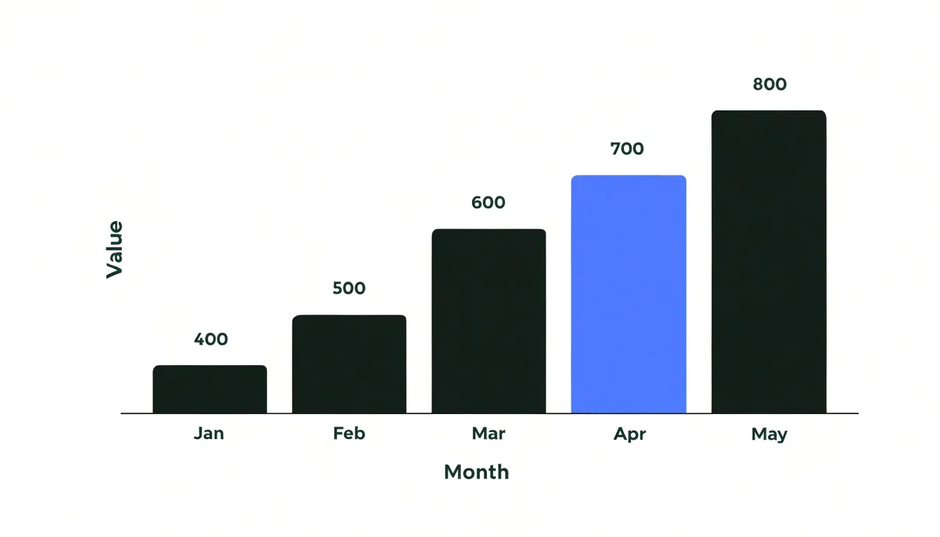
Table of Contents
Bar Chart
The bar chart is the workhorse of categorical comparison, translating discrete group counts into lengths the eye can rank almost instantly. Each bar should encode one category along the baseline, with the value axis starting at zero so that bar lengths remain proportional to the quantities they represent. Sorting the bars by value—rather than alphabetically or by arbitrary group order—lets readers perceive rank order without scanning back and forth between labels and lengths. Keeping the gaps between bars modest and uniform preserves the visual integrity of each quantity. Use a single color for all bars to keep attention on the comparison, reserving a highlight color for the category that carries the main finding, and use direct labels where possible instead of a separate legend that forces the eye to travel.
The choice between vertical and horizontal orientation often follows from the labels:
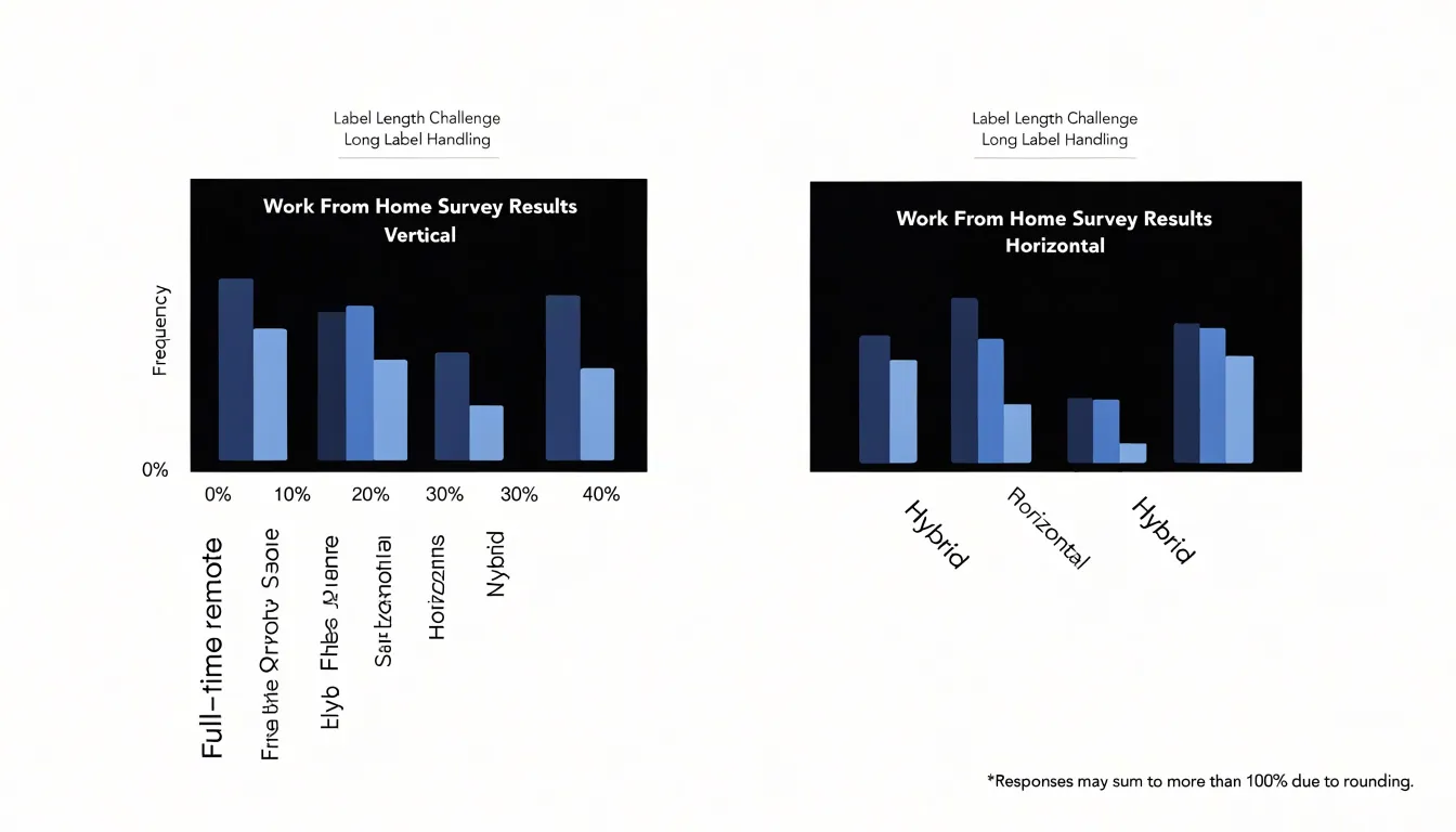
- Vertical bars suit short category names such as months, quarters, or brief group codes, mirroring the familiar chronological left-to-right reading pattern.
- Horizontal bars work best when category labels are long or numerous, such as survey items, department names, or multi-word audience segments. Laying the chart on its side gives each label a full line of horizontal text, eliminating rotated, angled, or truncated text. Horizontal layouts also scale gracefully for fifteen or twenty categories, since the bars can stack down the page without squeezing the width.
The rule of thumb is simple: when labels threaten to tilt, rotate, or collide, flip the chart so the categories run vertically beside their bars.
Line Chart
A line chart is the standard choice for tracking trends over time because it maps a continuous chronological sequence onto a continuous visual path. The horizontal axis carries time, ordered from earliest to latest, while the vertical axis carries the measured value. Each observation becomes a point at the intersection of its timestamp and value, and a line connects consecutive points in sequence. That connecting line turns a scatter of individual readings into a readable trajectory, showing direction, momentum, and turning points at a glance.
Plotting continuous chronological datasets effectively begins with honest spacing. When time intervals are uniform, points can be spaced evenly along the axis. When intervals vary, the axis should reflect actual elapsed time so that collection gaps do not distort the apparent rate of change. Match the cadence of data points to the natural rhythm of the phenomenon: daily readings suit fast-moving metrics, while weekly, monthly, or quarterly intervals serve slower processes and reduce noise.
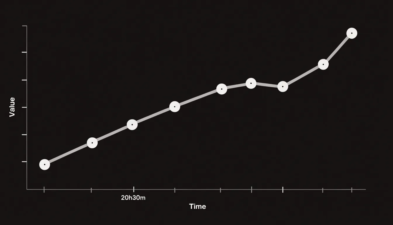
The number of points along the line also shapes interpretation. Too few points produce a jagged path that overstates volatility, while a dense series smooths the curve and reveals the macro-level direction. Choosing an appropriate time interval is a balancing act between responsiveness and clarity; aggregating fine-grained data into meaningful periods often exposes the trend that individual readings hide. The slope of the line communicates growth or decline, while crossings and plateaus mark shifts in behavior.
Pie Chart
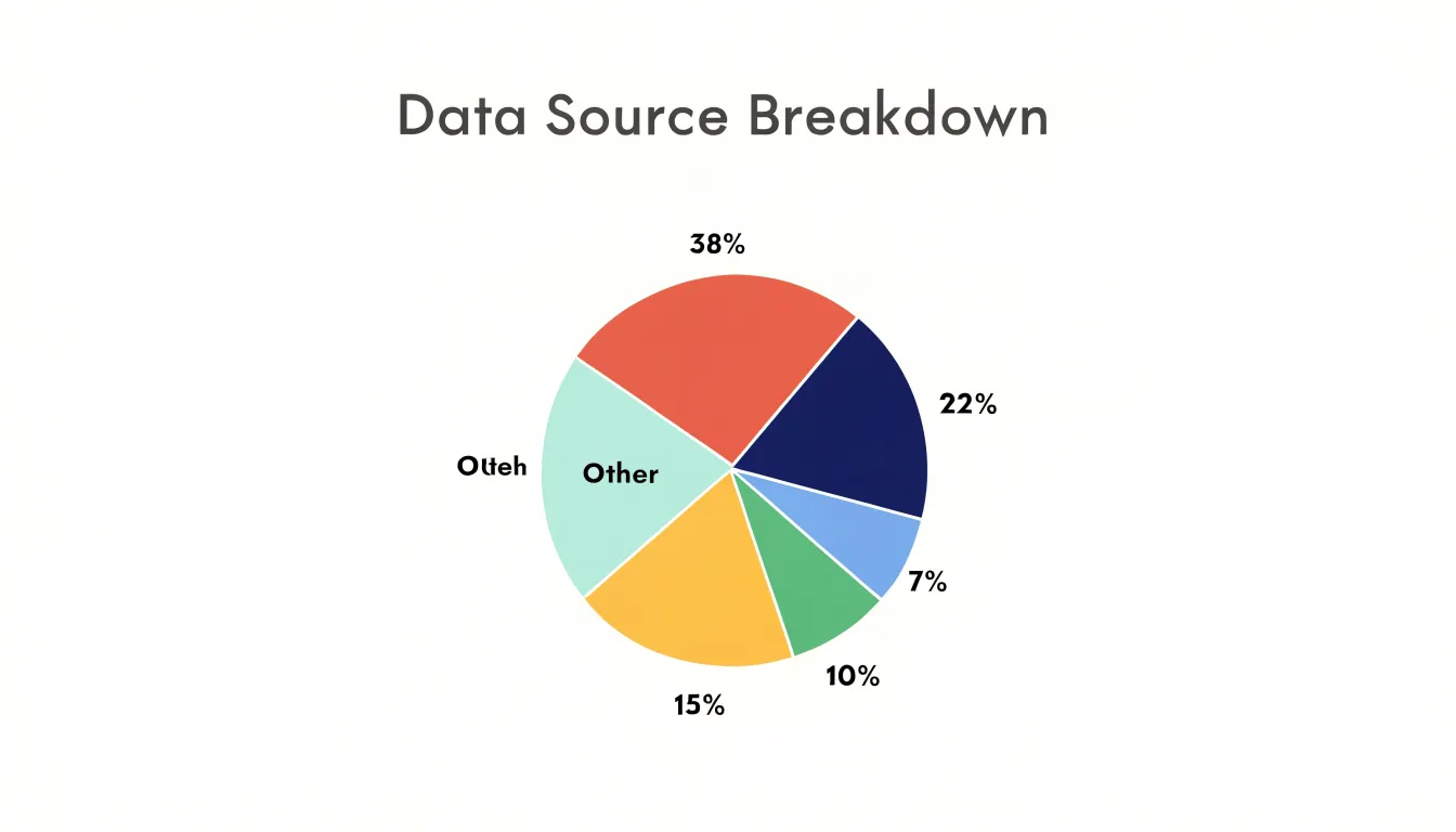
Pie charts show how individual parts combine to form a whole, with every slice representing a share of a single total that adds up to 100 percent. This makes them well suited to proportional breakdowns where the audience needs to grasp relative size at a glance, such as market share held by competitors, a budget divided across departments, or the share of survey respondents choosing each answer. Because the circle stands for the entire category being measured, the format works best when the underlying data genuinely forms a single unified whole and the number of categories is small.
A practical guideline is to limit the chart to roughly five to seven slices, grouping any smaller categories into a single slice labeled “Other.” Beyond this range, segments become narrow and similar in size, making it difficult for viewers to judge angles and areas accurately or to distinguish one wedge from another. Ordering slices by size, starting from the largest at the top and moving clockwise, gives the eye a natural path to follow and reinforces the ranking of categories. Placing clear labels directly on or near each slice further reduces the effort required to read the chart.
Scatter Plot
A scatter plot places one numerical variable along the horizontal axis and another along the vertical axis, turning each observation into a single point at the intersection of its two values. This direct positional mapping reveals relationships between variables:
- Upward diagonal cluster: Higher values on one axis tend to accompany higher values on the other, indicating a positive correlation.
- Downward diagonal cluster: One variable rises as the other falls, suggesting a negative correlation.
- Shapeless cloud: Signals little or no relationship.
Readers can assess both the strength of the pattern and its shape, including whether the association curves rather than follows a straight line. Adding a trendline makes the direction and steepness of the relationship easier to read. A simple linear fit summarizes the overall slope, while a curved fit captures nonlinear patterns. Trendlines also help distinguish genuine structure from random noise in dense distributions, where thousands of overlapping points can obscure the underlying shape. To handle overplotting and keep crowded regions legible, use transparency, smaller point sizes, and density-based coloring.
Spotting statistical outliers is another core strength of the scatter plot. Points sitting far from the main cluster or well away from the fitted trendline deserve investigation, as they may represent data entry errors, rare events, or genuinely distinct subgroups. Because outliers are identified visually in two dimensions at once, a scatter plot can reveal cases that summary statistics alone would hide. Proper axis scaling, point opacity, and reference lines for expected ranges all support careful reading of these distributions.
Color Choices
Color guides the eye before the reader has processed a single number. A well-chosen palette creates order: related categories share a family of hues, hierarchical levels step gradually from light to dark, and the most important data point stands out immediately. Harmony can be achieved with a few dependable approaches:
- Analogous schemes: Built from neighboring hues on the color wheel, these feel calm and unified, suiting dashboards where many charts appear together.
- Monochromatic ramps: Varying only in lightness, these work especially well for sequential data such as rates or totals, since readers intuitively read darker as larger.
- Muted complementary colors: A restrained set offers contrast without visual noise when a chart needs to distinguish a handful of unrelated categories.
A palette should reserve its strongest color for the finding that matters most, letting a single highlighted bar, line, or region carry the message while supporting elements recede into soft grays and desaturated tints. This keeps attention focused and reduces reliance on annotations. Backgrounds, gridlines, and axes also benefit from low-saturation tones that quietly frame the data rather than compete with it.
Avoid placing saturated neon tones and fully intense hues side by side. They create glare—especially on bright screens viewed for long periods—tire the eye, and flatten hierarchy because every element shouts at the same volume. Large areas of pure red or electric blue can also distort perception of the underlying values and make comparisons harder.
Color Accessibility
A meaningful share of any audience perceives color differently from the designer. Red-green color blindness (deuteranopia or protanopia) is the most common form, affecting a substantial portion of men and a smaller share of women. It collapses distinctions that many default palettes depend on, making a red bar next to a green bar look nearly identical. Blue-yellow deficiencies and reduced overall color sensitivity create similar risks for palettes built on those hues.
High-contrast color schemes offer a primary line of defense. Palettes that vary strongly in lightness as well as hue stay distinguishable even when hue information is lost, because the eye still registers the difference between a pale tint and a deep shade. Designers can use simulation tools to preview a palette under different color vision deficiencies and run lightness checks to confirm that adjacent colors remain separable. Limiting the palette to a few well-separated hues further reduces the chance that two categories will collide.
Secondary indicators provide a second line of defense by encoding information through channels other than hue:
- Distinct fill patterns such as hatching, dots, or diagonal lines let readers tell series apart by texture.
- Direct labels placed on or beside data points remove the need to match colors against a legend.
- Varied marker shapes, line styles (solid, dashed, dotted), and consistent category ordering reinforce the distinctions the colors carry.
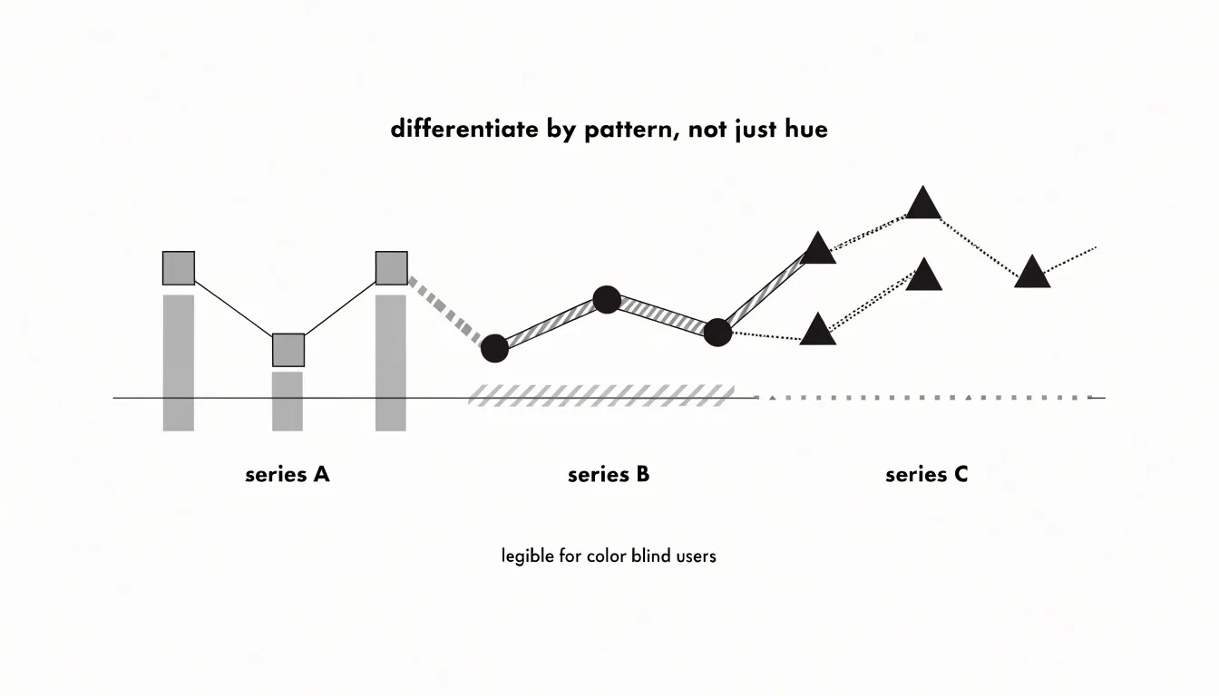
Used together, lightness contrast and secondary encoding keep a chart legible across a wide range of visual abilities, making the result clearer for every reader.
Data Labels
Data labels attach specific numeric values directly to chart elements, turning a general visual impression of shape and position into a precise reading. Surfacing exact figures on or beside critical data points gives audiences the confidence to quote a number, compare two values directly, or act on a threshold without consulting a separate table.
The challenge lies in selectivity: labeling every element makes a chart noisy and hard to scan. Instead, label only the points that carry the story, such as endpoints, peaks, outliers, targets, and values a decision depends on. Automated label placement routines in charting libraries reduce overlap through collision detection—nudging annotations outward, repositioning them above or beside markers, or adding leader lines that connect a distant label to its point in crowded clusters. Even so, a final manual review catches cases an algorithm misplaces.
Formatting choices reinforce clarity. Use consistent decimal precision, state units once in a header or axis title, and apply a subdued font weight, smaller text size, or lighter color so labels read as annotations without competing with the data marks.
Axis Scales
As noted with bar charts, the visual length or area of graphical elements must remain proportional to the data values they represent. If a bar chart’s vertical axis starts at 90 instead of 0, a bar representing 100 will appear only one-tenth the height of a bar representing 200, severely exaggerating the difference. While bar and area charts require a zero baseline because their encoding relies on length or area from a common starting point, line charts can sometimes use non-zero baselines to highlight small fluctuations over time—though this should be used with caution and clearly indicated.
Non-linear scales, such as logarithmic scales, present additional challenges. Logarithmic scales compress large ranges and reveal patterns in data that span orders of magnitude, but they distort spatial perception because equal distances on the axis represent multiplicative rather than additive changes. Viewers may misinterpret the steepness of a curve or the size of differences. To prevent misreading:
- Label the axis clearly to indicate it is logarithmic and show actual values at tick marks.
- Explain why a logarithmic scale is used in the chart title or annotations.
- Add gridlines at meaningful intervals to help viewers gauge magnitudes.
- Use a linear scale for audiences unfamiliar with logarithmic representations when possible, or offer a secondary linear view.
Layout and White Space
Layout and white space shape how a reader moves through a visualization. Generous outer margins frame the chart as a self-contained object and separate the data area from titles, captions, and legends, while tighter internal spacing groups related elements—such as axis labels and tick marks—into readable clusters. The balance between these two scales of spacing determines whether a chart feels crowded or composed.
Visual hierarchy gives the reader a clear sequence to follow. Size, weight, color intensity, and position signal importance, drawing attention to the largest and most contrasting elements first. A bold headline, a slightly smaller subtitle, and lighter annotation text create tiers that let the reader absorb the main message at a glance before descending into detail. Axis lines and gridlines belong low in that hierarchy, visible enough to support reading values without competing with the data marks.
Strategic alignment reinforces this order. Shared edges, consistent baselines, and aligned labels create invisible paths the eye follows naturally. When elements snap to a common grid, the layout reads as intentional, and deviations stand out as meaningful rather than accidental. White space—the gaps between bars, padding around callouts, and empty regions at the edges of a plot—gives the eye resting points and acts like a spotlight around key takeaways.
Common Chart Mistakes
Misleading visualizations often stem from design choices that distort factual accuracy:
- Truncated axes: Starting a vertical scale above zero makes small changes appear dramatic—for example, starting a bar chart at 90 instead of 0 can make a 2% increase look like a doubling. Always check whether the axis origin implies a magnitude the data does not support.
- Unnecessary 3D elements: Adding depth to pie or bar charts introduces perspective distortion. In 3D pie charts, front slices appear larger than back slices of equal value, and the added dimension makes it harder to compare areas and angles accurately. Flat, 2D designs are more truthful and easier to read.
- Improper metric aggregations: Summarizing data carelessly can hide variation or create false trends. Averaging percentages across groups of different sizes produces a misleading overall average, as does summing data that should be averaged (or vice versa), or combining data from different time periods and categories without adjustment. Always verify that the aggregation method matches the question being asked.
Data Preparation
Data preparation turns raw numbers into trustworthy inputs through three fundamental cleaning steps:
- Address null values: Missing data points can collapse gaps, skew averages, or produce broken lines in a trend. Decide deliberately whether to remove incomplete rows, substitute a documented placeholder, or carry values forward where the business context supports it, and record how gaps were handled.
- Standardize date formats: Dates arrive as text strings, serial numbers, regional day-month orderings, or timestamps with inconsistent time zones. Without a single canonical format, a time-series chart can render points out of sequence or scatter records across the wrong axis. Convert every date field into one consistent representation and verify that calendar values were preserved.
- Filter outliers: Extreme values can flatten the rest of a chart near zero or stretch an axis until patterns disappear. Review unusual records to confirm whether they reflect genuine events (like a bulk order) or system errors, then decide whether to exclude, cap, or annotate them. Always document any excluded legitimate extremes alongside the chart.
Audience-Centered Design
Good design adapts complexity, chart types, and framing to the reader’s context and purpose:
- Executives scanning a quarterly review need the headline insight within seconds. Their visuals should rely on clear, single-message charts (such as a single bar chart for a steering committee) with a strong title stating the takeaway, minimal clutter, direct labeling, and a tight palette highlighting the key number. Keep technical depth low, translate jargon into plain language, and move supporting detail to an appendix.
- Analysts want to interrogate the data themselves. They benefit from denser displays (such as small-multiple grids or scatterplot matrices), finer granularity, confidence intervals, annotated anomalies, and consistent axes for cross-view comparison. Domain terminology like statistical significance or cohort retention can be used freely.
Before building a chart, write a one-sentence statement defining the audience and the decision the visual supports, then let that guide your labeling, aggregation level, and inclusion of raw values. When a single deliverable serves multiple groups, use layered views—such as an executive summary slide followed by detailed dashboards, or on-demand technical annotations. Finally, review drafts with a representative reader to catch mismatches in depth and terminology.
Interactive Elements
Interactive elements keep the initial view uncluttered while offering depth on demand for user-driven exploration:
- Hover details (tooltips): Moving a cursor over a data point can trigger a dynamic tooltip showing precise values, labels, percentage changes, period comparisons, or contextual notes that would clutter a static view.
- Drill-down capabilities: Clicking a high-level summary element—such as a bar in a regional sales chart—can reveal a finer breakdown by city or product category, letting users explore hierarchies at their own pace.
- Filtering toggles: Checkboxes or dropdown menus let users slice the view by time range, category, or geography, updating the chart instantly to answer specific questions.
Dashboards
A dashboard combines several visuals so a reader can assess the state of a business in a single glance. Place the most important numbers—such as metric cards carrying a single headline figure—at the top left where the eye lands first, with supporting charts flowing outward and downward to explain movement or breakdowns. Group related panels into bands by shared context (for example, separating revenue visuals from customer visuals) so viewers can build a quick mental map of the layout.
Consistent panel sizing, alignment, modest gutters of white space between tiles, and repeated axis conventions reduce the mental effort of moving from one chart to the next. Give filters and controls a permanent home, usually a persistent top strip or side rail, so their placement never shifts and their effect on every panel remains clear. If the dashboard is interactive, use cross-filtering and linked highlighting so users can trace a single selection across the entire view. A stakeholder should be able to open the dashboard, read the headline metrics, and locate the one or two charts explaining an anomaly within seconds.
Frequently Asked Questions
Should a bar chart’s value axis start at zero?
Yes—the article says each bar should encode one category with the value axis starting at zero so bar lengths remain proportional to the quantities. It also states that bar and area charts require a zero baseline because their encoding relies on length or area from a common starting point.
How many slices should a pie chart have?
A practical guideline is to limit the chart to roughly five to seven slices, grouping any smaller categories into a single slice labeled “Other.” Beyond that range, segments become narrow and similar in size, making them difficult to judge accurately.
How do I choose the right time interval for a line chart?
Match the cadence of data points to the natural rhythm of the phenomenon: daily readings suit fast-moving metrics, while weekly, monthly, or quarterly intervals serve slower processes and reduce noise. The article notes that too few points produce a jagged path that overstates volatility, while a dense series smooths the curve.
How can I spot outliers on a scatter plot?
Points sitting far from the main cluster or well away from the fitted trendline deserve investigation, as they may represent data entry errors, rare events, or genuinely distinct subgroups. A scatter plot can reveal these cases visually in two dimensions at once.
How can I make a chart accessible to people with color blindness?
Use high-contrast color schemes that vary strongly in lightness as well as hue, and limit the palette to a few well-separated hues. Add secondary indicators such as distinct fill patterns, direct labels, varied marker shapes, and different line styles to reinforce distinctions.
When can a line chart use a non-zero baseline?
Bar and area charts require a zero baseline, but the article says line charts can sometimes use non-zero baselines to highlight small fluctuations over time—though this should be used with caution and clearly indicated.
Tony Astor
Tony writes about data visualization and the tools people use to build charts and dashboards. More about Data Illustrator