Data-Ink Ratio: Tufte's Principle Explained
 By Tony Astor ·

Data-Ink Ratio
The data-ink ratio is the proportion of a chart’s total ink used to display actual data values, calculated as data ink divided by total ink. Introduced by Edward Tufte, it measures chart efficiency: a ratio near 1.0 means almost all ink encodes data, while values near zero indicate clutter from gridlines, borders, and decoration.
Table of Contents
The Core Concept
The data-ink ratio is a quantitative measure of chart efficiency, defined as the proportion of ink used to display actual data values relative to the total ink used to render the entire graphic. In practice, this means adding up everything the chart draws—including axis lines, tick marks, gridlines, labels, borders, background fills, and decorative elements—and comparing that total against the ink consumed solely by the data-bearing marks themselves. The result is a simple fraction: data ink divided by total ink. A chart where every drop of ink carries information approaches a value of one, while a chart cluttered with ornamentation and redundant lines falls toward zero. Edward Tufte, who introduced the concept, framed the goal as devoting the maximum possible share of ink to genuine data points and the minimum to everything else.
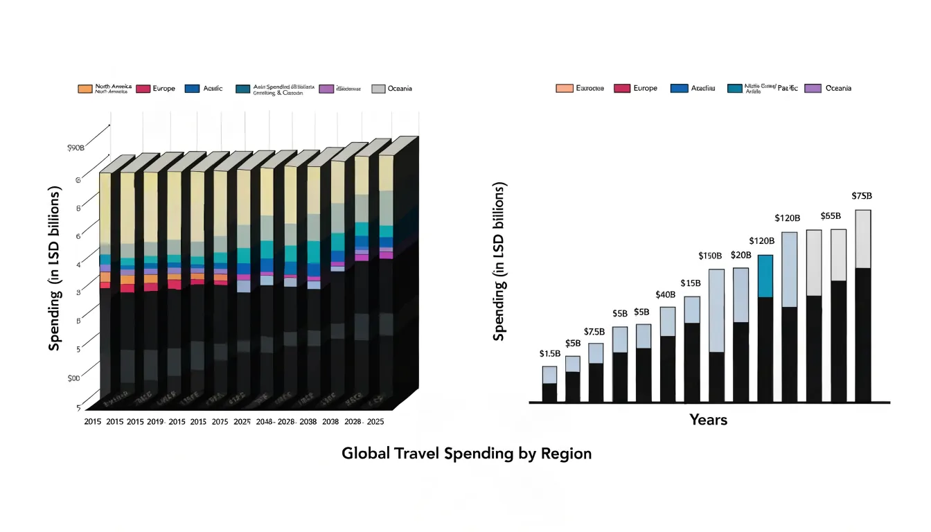
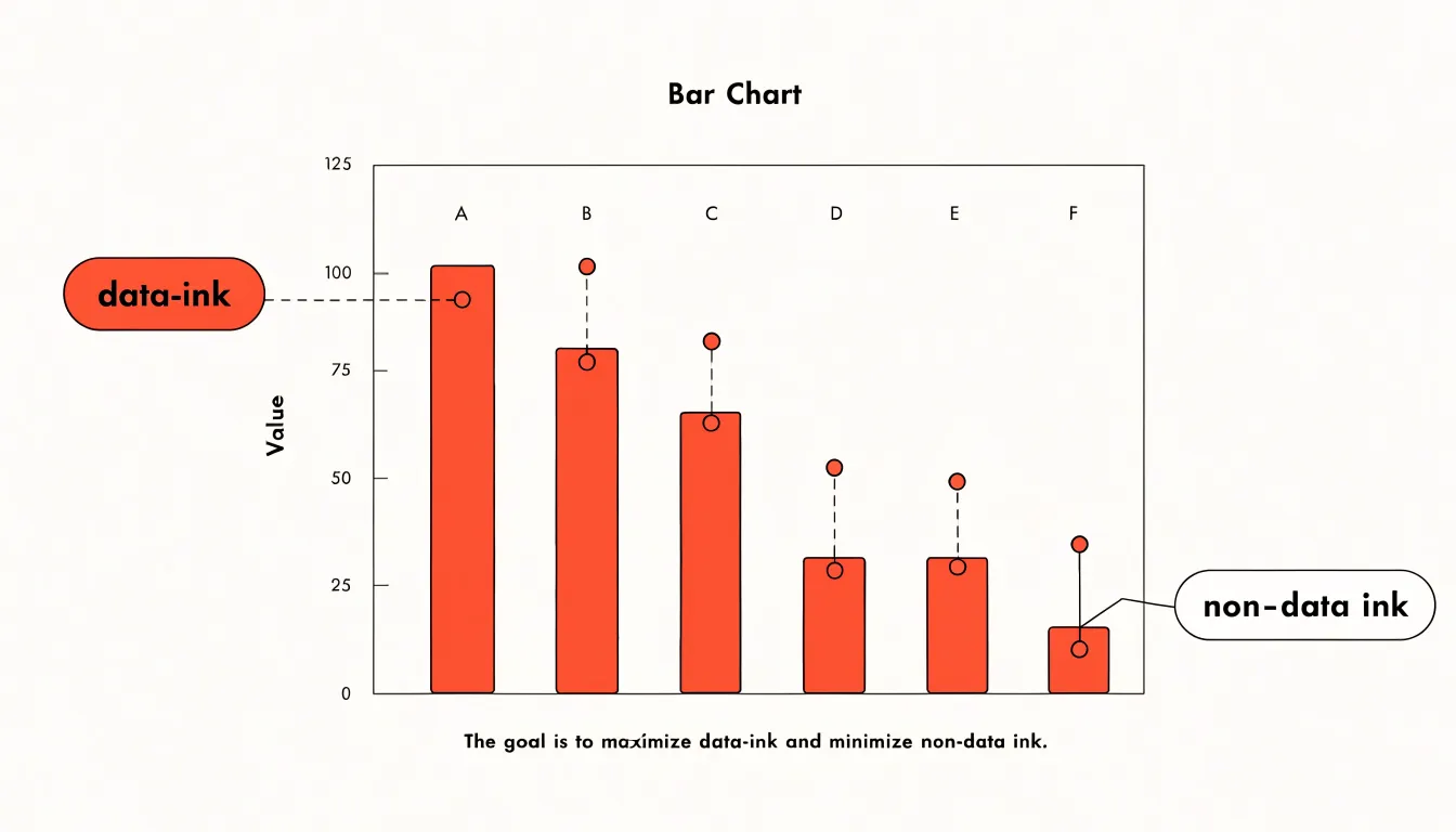
The visual definition rests on identifying which marks actually encode values. A bar, a line segment, or a plotted symbol whose height, position, or length corresponds to a number counts as data ink. Structural elements that merely frame or organize the display count as non-data ink. The ratio captures the balance between these two categories. Striving for a high ratio means erasing gridlines that add no interpretive value, removing heavy borders, dropping unnecessary backgrounds, and trimming labels to what the viewer genuinely needs. Each reduction transfers emphasis back to the data. The principle does not demand the lowest possible ink overall, since some structural ink aids comprehension, but it does insist that every mark justify its presence by communicating information. Readers gain clarity when visual weight flows toward the numbers rather than toward the frame around them, and the ratio offers a concrete way to check that the graphic’s ink budget supports that outcome.
Defining Data Ink
Data ink refers to the marks on a chart that directly represent quantitative information—the bars in a bar chart, the line in a trendline, the points in a scatter plot, the segments of a pie chart, or the area under a curve. These visual elements encode the actual numbers, proportions, or relationships in your data.
To identify essential chart elements, start by asking a simple question: if this mark were removed, would the viewer lose access to a data value? For a bar chart, the height or length of each bar is essential because it corresponds to a magnitude. For a trendline, the line’s position and slope convey change over time. For a scatter plot, each point’s location on both axes represents a pair of values. These marks are the primary carriers of meaning. Other elements, such as gridlines, axis lines, tick marks, and labels, serve supporting roles—they help interpret the data but do not themselves represent quantitative values. They may be necessary for context, yet they are not data ink in the strict sense.
Data ink also includes less obvious elements that still encode data directly:
- In a stacked bar chart, each segment’s height is a data value.
- In a dot plot, each dot’s position along the axis is a data point.
- In a heatmap, the color intensity of each cell corresponds to a value.
- Error bars, which show uncertainty, are data ink because they convey quantitative information about variability.
Spotting Non-Data Ink
Non-data ink is any mark on a chart that does not encode a value or help the reader decode one. Background fills are among the most common offenders. A soft gradient or shaded panel behind a bar chart may look polished in a mockup, yet it adds visual weight without carrying information; the reader’s eye must work past the tint to reach the bars. Replacing the fill with plain white, or a very light neutral when grouping demands separation, restores focus to the data itself.
Decorative icons present a similar problem. A little illustration beside a chart title, or pictograms repeated across a dashboard, can multiply into a field of competing shapes that draw attention away from the plotted marks. Icons work best when they substitute for data marks, as in an isotype chart, and become clutter when they merely ornament.
Duplicate tick marks deserve particular attention because they hide in plain sight. A gridline and an axis tick often convey the same reference point twice, so one of them can go. Ticks drawn along the top and right edges of a plot, mirroring those on the bottom and left, add nothing for the reader who already has the primary axes. Minor gridlines in five-step intervals, when labels appear only at major intervals, create a dense mesh that competes with the data line. Each of these elements is small on its own, but together they slow reading.
Spotting such elements is largely a matter of habit. Cover each visual feature in turn and ask whether any information is lost, or count how many distinct marks serve one piece of information, since duplicates signal redundancy.
Calculating the Ratio
The data-ink ratio gives you a concrete number to work with rather than relying on vague impressions of clutter. A chart that uses 100 units of ink and dedicates 80 of them to encoding values has a ratio of 0.8. The closer that number gets to 1.0, the more efficient the graphic. Anything well below that threshold signals room for improvement, and the arithmetic itself is simple enough to do informally with your eye once you have practiced the estimate.
What matters more than the exact figure is the systematic audit the formula encourages. Before publishing any graphic, work through it in stages:
- Identify every mark on the page and ask whether it represents a data value. List the non-data elements, then decide which ones can be removed without loss of meaning.
- Look at the marks that do encode data and check whether they are doing so efficiently, such as thick bars that could be thinner or overlapping elements that obscure their own values.
- Perform a subtraction pass: try removing one element at a time and ask whether the chart still communicates the same message. If it does, leave it removed.
Consistency in applying this routine matters more than the precision of your mental ratio estimate, because repeated small removals accumulate into visibly cleaner, faster-to-read graphics.
Reducing Visual Noise
Every mark on a chart competes for the reader’s attention. The human visual system processes a scene in two broad stages: a fast, parallel pass that picks out salient features like color, position, and size, followed by slower, serial attention that examines specific elements one at a time. Any decorative or non-essential ink enters that first pass as a candidate for attention, and the reader must expend effort to ignore it. Because working memory holds only a handful of items at once, each irrelevant element that slips through consumes capacity that would otherwise go toward interpreting the data itself.
This burden shows up behaviorally. Eye-tracking studies of chart reading consistently find that viewers fixate longer and revisit regions more often when grids, borders, heavy labels, and ornamental backgrounds are present. Those fixations do not translate into better understanding; they reflect search effort. The reader is working to separate signal from noise, delaying comprehension. In practical terms, a cluttered chart asks the audience to perform a sorting task before they can perform the actual comparison the chart was built to support.
The effect compounds with task complexity. Simple lookups of a single value survive mild clutter, but comparisons across categories, trend judgments, and estimates of proportions degrade quickly as extraneous ink accumulates. Decision-makers scanning a dashboard under time pressure are especially vulnerable, since they rely on rapid perceptual judgments that clutter disrupts. Preattentive cues like a single accent color or a clear positional ordering get drowned out when competing visual elements crowd the display. Removing these distractions lowers the perceptual cost of reading, shortens the path from glance to judgment, and leaves working memory free for reasoning.
Removing Chartjunk
Heavy gridlines and dark borders are among the most common sources of chartjunk, and they are often the easiest to remove. In many charting tools, the default settings produce a black frame around the plot area and a dense lattice of dark gray gridlines that compete directly with the data. The eye is drawn first to the strongest contrasts in an image, so when the frame and grid are rendered in near-black while the data marks are lighter, the structural scaffolding becomes the visual subject of the chart rather than the values it conveys.
Softening begins with the gridlines themselves. Dark gray or black gridlines can typically be replaced with a pale gray, a dotted or dashed line, or a significantly thinner stroke. The goal is a texture faint enough that it recedes when viewed casually yet can still be followed when a reader wants to trace a value across the plot. Where the chart allows it, removing horizontal gridlines while keeping the ones that align with axis labels, or vice versa, reduces clutter while preserving orientation. In some cases a single set of gridlines is enough, and the redundant set can be dropped entirely.
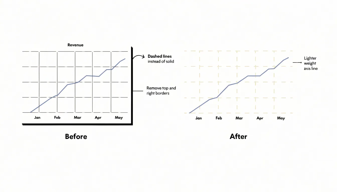
The enclosure lines deserve similar treatment. A full box around the plot area often adds four strokes that carry no information. Removing the top and right segments, leaving only the axis lines that anchor the labels, keeps the chart legible while opening up the visual field. The remaining axis lines can be lightened or shortened so they end at the final tick rather than extending past the data. Tick marks themselves can also be reduced in number or length to remove small visual interruptions along the axes.
Redundant structural markings extend to borders around legends and decorative lines separating titles or captions. Each of these elements can be eliminated or rendered in a lighter shade, allowing the marks that represent actual data to carry the full weight of the visual contrast.
Rethinking 3D Effects
Adding depth to a bar or a pie slice may appear to lend a graphic sophistication, yet the moment perspective is introduced, the geometry that governs how values are read shifts in unintended ways. A bar rendered with a receding front face and a far edge occupies more pixels on the screen than its numeric value warrants, and the viewer’s eye cannot easily separate the extra visual bulk from the quantity it is meant to encode. The length of an element no longer corresponds reliably to the number it represents, turning the reading of proportion into guesswork rather than measurement.
The distortion is most acute in pie charts drawn at an angle. A circular pie sliced into equal parts offers a direct visual correspondence between each slice’s angular sweep and its share of the whole. Tilt that pie backward, and the slices at the front appear larger while those at the rear compress toward the top of the ellipse. Two categories with identical values can end up looking markedly different in size, with no cue that the discrepancy is an artifact of the rendering rather than a feature of the data. Even modest perspective effects introduce this bias, and the more pronounced the angle, the further the visual proportions drift from the underlying numbers.
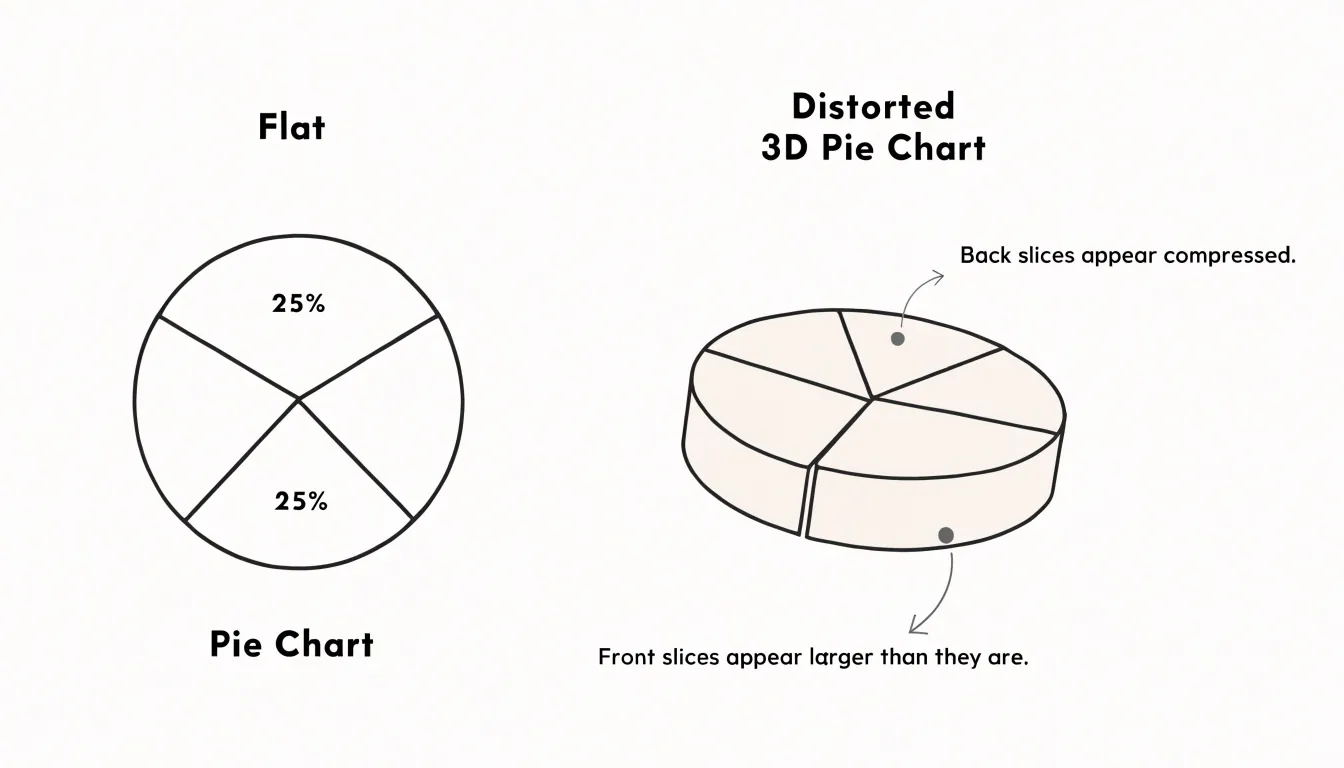
Flat two-dimensional designs avoid this problem entirely. When every element is drawn on the same plane, area and length map straightforwardly onto value. A bar of twice the height represents twice the quantity, and a wedge spanning 90 degrees represents a quarter of the total. Readers can compare segments directly without mentally correcting for foreshortening, while removing the third dimension also strips away decorative shading and extraneous faces that consume ink without carrying information.
Smart Color Choices
A frequent culprit in cluttered charts is the rainbow palette, where each category receives a different saturated color with no relationship among them. The eye darts from red to green to purple without knowing where to settle, and the reader spends cognitive effort decoding colors that convey no information beyond mere identity.
A more disciplined approach begins with a monochromatic scale, where a single hue varies in lightness or saturation to encode magnitude. Because the human visual system reads ordered steps of one color as an ordered progression, a sequence of blues from pale to deep communicates low-to-high values intuitively, letting the reader grasp the gradient at a glance.
Where differentiation among a few categories is genuinely needed, targeted accent colors serve better than a full spectrum. By rendering the bulk of the graphic in neutral grays or muted tones and reserving one or two strong colors for the elements that matter, the designer creates a clear visual hierarchy. A single bold accent can spotlight a trend line, flag an outlier, or highlight the category under discussion, effectively telling the viewer where to look first. Shades within a family or a small set of purposeful accents will nearly always outperform an arbitrary multicolor scheme in clarity and focus.
Labeling Directly
Direct labeling places descriptive text right beside the data it identifies, so a line at the top of a chart carries its own name at that endpoint, and a bar carries its value at the tip. The alternative is the familiar legend: a small key set off in a corner or along an edge, mapping colors or symbols to series names. Every time a reader wants to know which line is which, their eye must leave the plotted area, find the matching swatch in the legend, register the color, and travel back to the data. On a chart with several series, that eye travel happens repeatedly through the course of reading.
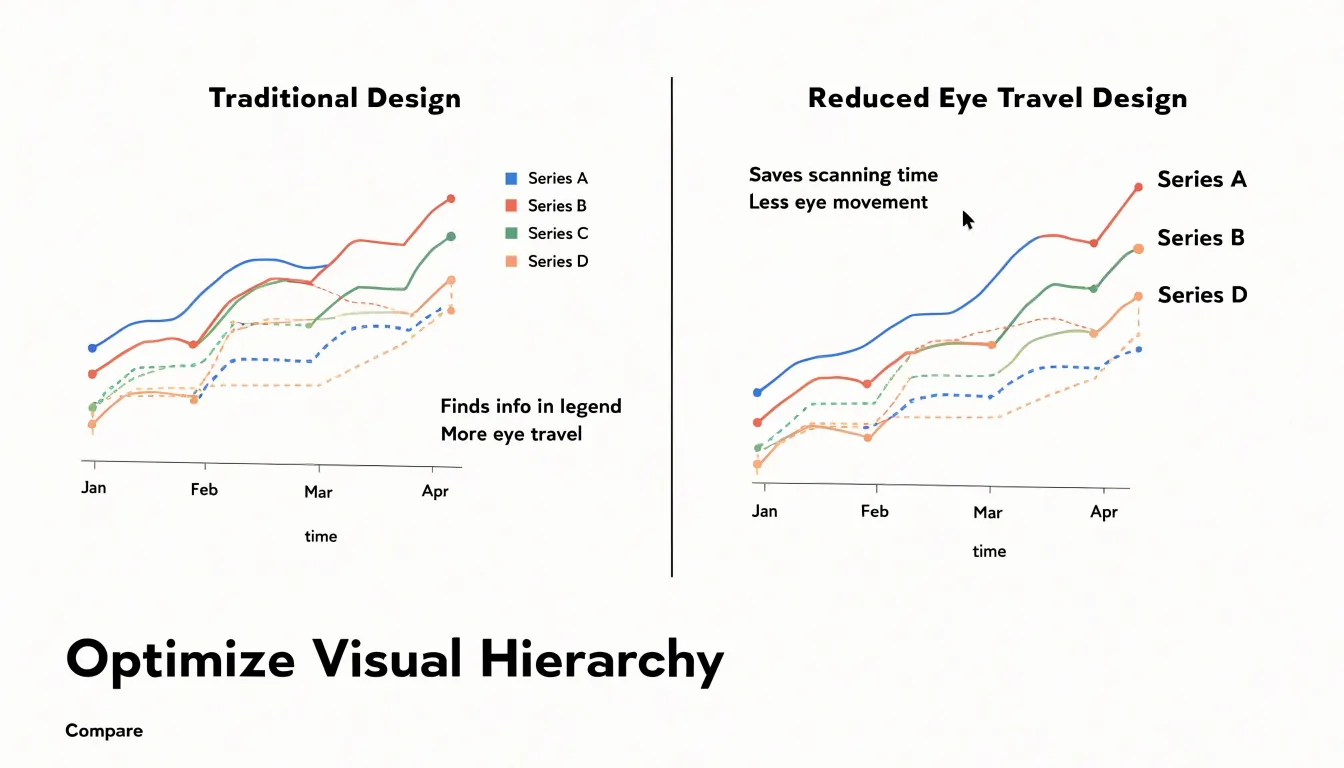
When the label sits adjacent to its series, recognition happens in a single glance. This is especially valuable when lines converge, cross, or run close together, since a nearby label can anchor identity at exactly the point of confusion. Values printed at the end of bars or points likewise let the reader extract quantities without scanning a separate axis or key.
Direct labeling also supports clarity for readers encountering the chart outside its original context—such as in a report, a slide, or a screenshot where surrounding prose is absent—and on mobile screens where a legend may occupy scarce space. Labels can be angled along a line, offset from a marker, or aligned to a bar end, so they reinforce the visual structure rather than clutter it. On charts where space is tight, the label may replace a legend entirely, reducing the total number of elements competing for attention.
Maximizing Information Density
The data-to-space ratio is a simple accounting of how much of the visible area communicates actual values versus how much is devoted to decoration, padding, and empty framing. A chart that devotes half its canvas to heavy grid lines, ornate borders, and generous whitespace around a single trend line delivers a poor ratio; the viewer pays for space that returns no information.
One effective strategy is compression within the mark itself. Edward Tufte’s sparklines demonstrate how a small, word-sized graphic can encode a full time series in the space of a few characters of text. A sparkline might sit inline with a sentence, showing months of fluctuation in a strip no taller than a line of type. The technique works because it strips the chart to its essentials: the data path, perhaps a reference line, and an endpoint marker. Context is supplied by surrounding text rather than by redundant axes and labels.
Density also increases through layering related series in a single frame. Small multiples—repeated panels sharing identical scales—let viewers compare many datasets at once without repeating axis furniture for each one. Overlaying a reference band, a target line, or a shaded percentile range adds interpretive value at marginal spatial cost, provided the layers remain visually distinguishable through weight and tone.
The guiding constraint is comprehension. Density that forces the eye to labour is density wasted. Effective designers test their graphics at actual reading size, prune labels that can be moved to captions, tighten margins to the ink’s edge, and let typography do the work that boxes and rules once did.
Bar Charts
Because bar charts are so common, they tend to accumulate visual clutter—a full rectangular border, tick marks on both axes, gridlines running across the plot, and bars filled in heavy dark colors—without anyone noticing.
Removing the outer border opens up the chart and lets the bars breathe. On a vertical bar chart, the y-axis line and its tick marks often become redundant once the bars themselves are anchored to a shared baseline, and each bar can carry its own value label instead. Gridlines can be eliminated or lightened considerably, since the reader can compare bar heights directly against one another without needing a ruled background.
Solid black or saturated bar fills draw the eye toward the ink rather than the pattern in the data, and they make labels harder to read when placed inside or near the bars. Replacing these with lighter tones, or with a single consistent hue, keeps the chart visually calm while preserving the ability to distinguish categories through position and labeling.
Line Charts
Line charts excel at revealing trends over time, especially when stripped of excess lines and structural distractions. Beyond softening gridlines, simplifying axes, and labeling lines directly, several techniques help the trend emerge clearly:
- Use color sparingly: A single, bold color for the primary trend line draws attention, while secondary lines can be muted or grayed out.
- Emphasize key points selectively: Add data markers or annotations only where they add insight, such as peaks, troughs, or significant events.
- Limit the number of lines: If multiple series are shown, use small multiples or interactive filters to avoid a tangled plot.
- Adjust the aspect ratio: Time series often benefit from a wider format that makes slopes and trends more discernible.
Scatter Plots
Scatter plots reveal relationships that tables of numbers cannot show, yet default renderings often bury those relationships under visual noise. Cleaning up a scatter plot relies on three main levers:
- Point markers: Small, uniform, semi-transparent circles work well for dense clouds of data because overlapping marks build up darker regions that suggest local concentration, a phenomenon readers interpret intuitively. When one subgroup matters more than the rest, give it a slightly larger radius or a more saturated tone while keeping the others muted. Resist the temptation to encode every categorical variable with a different hue and shape combination; two or three visual distinctions usually exhaust a reader’s attention, and beyond that the legend becomes a lookup task rather than a guide.
- Reference lines: A thin, low-contrast horizontal line at a meaningful threshold, such as a target value or a historical average, or a diagonal line marking perfect agreement between two measures, lets readers judge deviations at a glance without competing with the data. Keep these strokes pale and unlabelled unless the label carries real interpretive weight.
- Callouts: Annotate a handful of outliers, clusters, or turning points with short text placed close to the point, connected by a leader line only when displacement is unavoidable. Each callout should answer a question the reader is likely to ask, such as which region or cohort sits apart from the trend.
Digital Dashboards
Digital dashboards have become the primary vehicle through which executives encounter data, and the tools that build them—Tableau, Power BI, Looker, and their peers—offer almost unlimited capacity for visual embellishment. Tufte’s data-ink principle translates directly into this environment: the pixels devoted to gradients, drop shadows, and non-data elements should be minimized, and the pixels that remain should be reserved for information that changes with the underlying numbers.
Applying the principle in business intelligence software begins with the chart type itself. Default templates often favor pie charts, gauges, and stacked bars where a simple line or sorted bar would communicate faster and with less ink. Executives scanning a dashboard under time pressure benefit from a small set of high-information charts, each labeled directly and stripped of redundant scaffolding so the eye lands on the trend or exception immediately.
Clutter removal extends to the surrounding interface. Dashboard headers, logos, filter panels, and navigation chrome all occupy space that could carry data. A disciplined executive view keeps controls minimal or tucked away, uses a restrained palette of two or three colors, and lets whitespace do the work of separation instead of heavy boxes and rules.
Modern tools also make it easy to over-populate: a dozen tabs, dozens of slicers, and KPI tiles stacked like a scoreboard. The data-ink lens suggests treating each dashboard as a single clear argument rather than a warehouse of every available metric. Building a clutter-free executive view is thus as much an editorial act as a technical one, and the tools reward that discipline when designers deliberately choose less.
Practical Action Steps
Before your next presentation, set aside twenty minutes to run any chart through a quick five-step audit:
- Identify every element on the chart: Note all bars, lines, points, axis lines, tick marks, labels, and plot borders. Listing them mentally or on paper builds the awareness needed for cleanup.
- Strip away decorative elements: Remove background fills, drop shadows, 3D effects, heavy gridlines, and ornamental borders that contribute nothing to understanding.
- Lighten remaining non-data elements: Recede gridlines into pale gray, thin or remove axis lines when labels make position obvious, and shorten or drop tick marks so the data marks carry the visual weight.
- Refine labels and typography: Check that axis labels are legible without dominating, state units once rather than repeating them on every tick, place data labels only where they add value, and replace legends with direct labels where possible.
- Step back and assess the overall balance: Squint at the chart and notice what draws your eye first. If a decorative element attracts attention before the data does, prune further, and test the chart at the actual size it will appear on screen.
Run these five steps on one chart today, then make the checklist a habit. Repeated practice turns the audit into a fast reflex, and your future graphs will communicate with steadily greater economy and force.
Frequently Asked Questions
What is the data-ink ratio in charts?
The data-ink ratio is the proportion of ink used to display actual data values relative to the total ink used to render the entire graphic. A chart where every drop of ink carries information approaches a value of one, while a cluttered chart falls toward zero.
How do you calculate the data-ink ratio?
Calculate it as data ink divided by total ink; for example, a chart using 100 units of ink with 80 dedicated to encoding values has a ratio of 0.8. The closer the number gets to 1.0, the more efficient the graphic.
What counts as non-data ink on a chart?
Non-data ink is any mark that does not encode a value or help the reader decode one, such as background fills, decorative icons, duplicate tick marks, and heavy borders. Gridlines, axis lines, tick marks, and labels may support interpretation but are not data ink in the strict sense.
Why should you avoid 3D effects in charts?
Adding depth changes how values are read, because a bar with a receding face occupies more pixels than its numeric value warrants and length no longer reliably corresponds to the number represented. The distortion is especially acute in angled pie charts, while flat two-dimensional designs map area and length straightforwardly onto value.
What color choices help reduce clutter in a chart?
Avoid the rainbow palette, where each category gets a different saturated color with no relationship among them, and begin with a monochromatic scale that varies in lightness or saturation to encode magnitude. Where differentiation is needed, render most of the graphic in neutral grays or muted tones and reserve one or two strong accent colors for elements that matter.
Should I use direct labels or a legend on a chart?
Direct labeling places descriptive text beside the data it identifies, so recognition happens in a single glance and the reader does not have to travel back and forth to a legend. On charts where space is tight, the label may replace a legend entirely, reducing the total number of elements competing for attention.
Tony Astor
Tony writes about data visualization and the tools people use to build charts and dashboards. More about Data Illustrator