Control Chart: How to Track Process Variation
 By Tony Astor ·

Control Chart
A control chart is a statistical process control tool that plots data over time against a center line and upper and lower control limits to separate common cause variation (normal process noise) from special cause variation (unexpected anomalies from outside sources). Points outside the limits or non-random patterns signal that investigation and corrective action are needed.
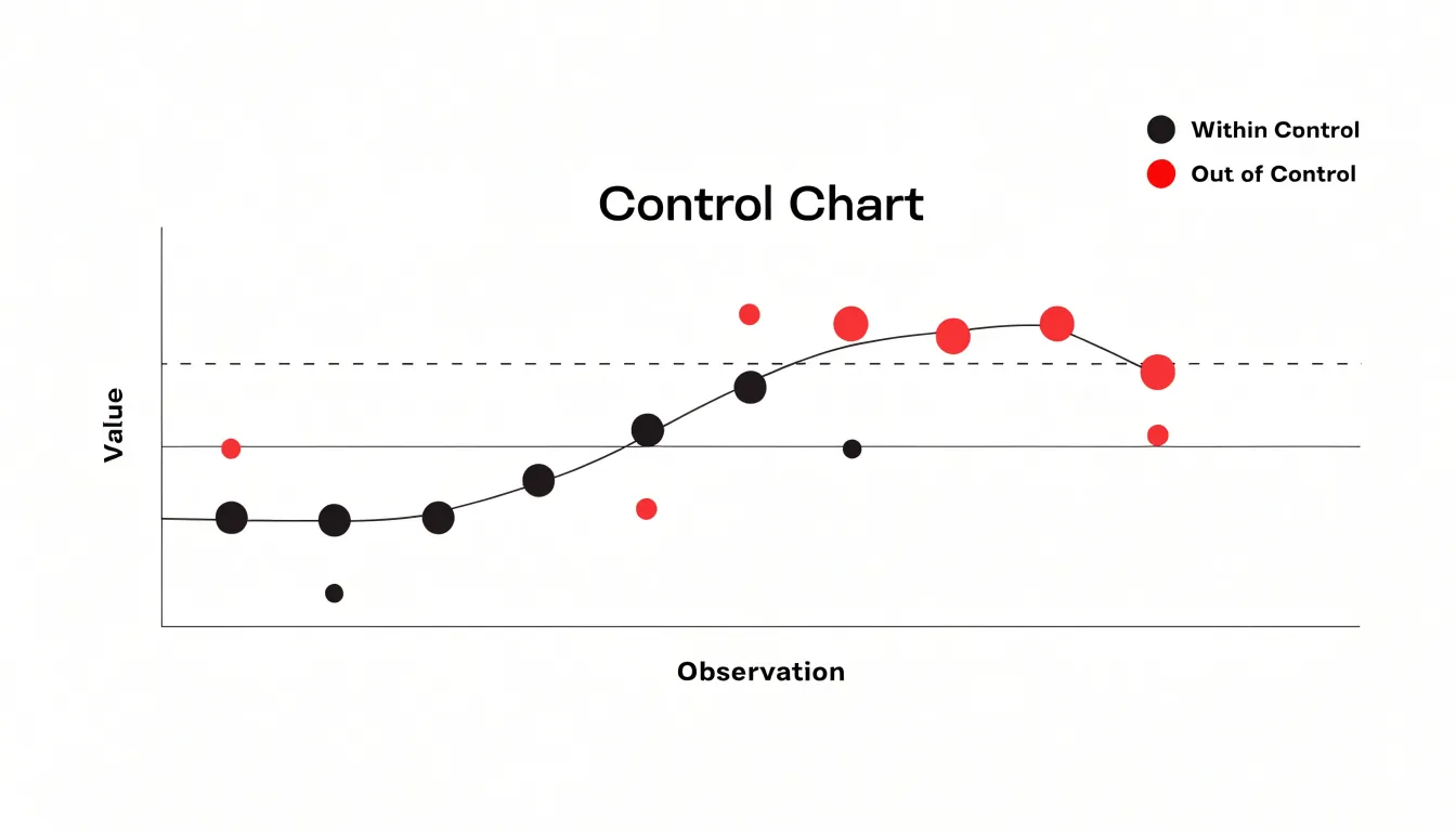
Table of Contents
- Control Chart
- Process Variation
- Common Cause Variation
- Special Cause Variation
- Control Limits and Center Line
- Choosing the Right Chart
- Gathering Sample Data
- Plotting Points
- Out of Control Signals
- Run Rule Patterns
- Baseline Limits
- Avoiding False Alarms
- Recalibrating Boundaries
- Common Tracking Mistakes
- Long Term Quality Control
Control Chart
Establishing a daily logging routine is the backbone of any control chart system. Operators should begin each shift by recording the same set of measures at the same time: extraction volume, temperature, pressure, and yield for every small batch. Consistency in when and how data is captured matters as much as the numbers themselves. A simple log sheet or digital form with pre-labeled fields reduces the chance of skipped entries and keeps the record comparable from day to day. Over time, this routine generates the baseline needed to recognize when a process drifts away from its normal range.

Small batch extractions deserve particular attention because they reveal variation quickly. Each batch should be logged with its start time, duration, and output weight, then plotted against the established target band. When a batch falls outside the expected limits, the operator notes the suspected cause in the log so patterns can be reviewed later. Tracking batches individually, rather than only daily totals, lets teams spot whether a single run or a recurring shift is responsible for a deviation.
Maintaining product standards across routine operations ties these practices together. The control chart works best when the defined limits reflect agreed specifications for the finished product, such as concentration, color, and moisture. Review the chart at a fixed interval, perhaps at shift handover, and mark any point that crosses a limit. Keep notes brief and factual so that the history stays useful for later analysis.
Process Variation
No two batches of essential oil are ever exactly alike, a natural consequence of the plants from which they are derived. Plants are living systems, and their chemistry responds continuously to the conditions in which they grow.
Biological factors play a central role: individual plants differ in genetics, age, and stage of development at harvest, and these differences influence how much of each compound the plant produces. A leaf harvested early in the season may carry a different balance of constituents than one taken weeks later, and even plants of the same species grown side by side can show measurable differences in their chemical makeup.
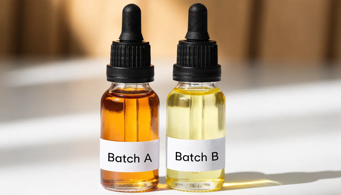
Environmental conditions add another layer of influence. Sunlight, temperature, rainfall, soil composition, altitude, and harvest timing all shape the plant’s metabolism and the profile of the oil it yields. A wetter growing season, a cooler summer, or a shift in soil minerals can each leave a subtle signature in the final product.
The practical result is minor natural variation across batches in aroma, viscosity, and chemical profile. One batch might smell slightly sweeter or more herbaceous than the last, pour a little more freely or thickly, and show small shifts in the relative proportions of its constituent compounds. These differences are generally small and fall within a natural range, meaning consistency is a matter of degree rather than an absolute. Distinguishing these normal batch-to-batch differences from meaningful deviations is the foundation of quality monitoring.
Common Cause Variation
Every production process carries a certain amount of natural movement. Outputs drift slightly from one unit to the next, measurements wobble around a central value, and small differences appear between shifts, machines, and operators. Quality practitioners call this ordinary ebb and flow common cause variation. It represents the background noise of a process—the sum of many small, essentially random influences built into how the system operates. A machining operation may leave microscopic differences in surface finish from one part to the next; a filling line may dispense volumes that vary by a fraction of a milliliter; a service desk may handle calls in times that differ by a minute or two. None of these fluctuations signals that something has gone wrong; they are the expected texture of a stable process.
When only common cause variation is present, individual results fall inside the tolerances engineers have established as acceptable. Reacting to each small deviation as though it were a problem tends to make things worse. Adjusting a machine because one unit came out slightly high, then readjusting because the next came out slightly low, introduces new disturbances and can actually increase the spread of results. This tendency, called tampering, is a frequent source of unnecessary variability.
Control charts plot data over time against statistically derived limits to separate this ordinary background noise from signals that demand attention. When only common cause variation is present, the appropriate response is to leave the process alone and, if improvement is desired, address the system as a whole rather than chase individual points.
Special Cause Variation
Special cause variation refers to unexpected anomalies arising from sources outside normal process operation. On a control chart, these appear as data points that fall outside the calculated control limits or form non-random patterns, signaling that an external factor has intervened. Unlike inherent, predictable common cause variation, special cause variation is intermittent and often traceable to a specific event.
Common examples include:
- Equipment malfunctions: A sudden temperature spike in a furnace or a motor failure on an assembly line.
- Raw material shifts: A new supplier delivering material with different properties.
- Environmental factors: Humidity changes or power fluctuations.
Once a chart flags a special cause, the next step is investigating the root cause by checking equipment logs, reviewing material certificates, or interviewing operators. Quick identification allows for timely corrective action, such as recalibrating a machine, isolating a batch of raw material, or adjusting environmental controls before anomalies corrupt batch quality, waste resources, or derail workflow.
Control Limits and Center Line
Every control chart rests on three horizontal reference points: a center line representing the process average, an upper control limit, and a lower control limit. The center line is calculated first, typically as the mean of the metric across a baseline period of stable production. For variables data such as cycle time or fill weight, this is often the arithmetic average of subgroup means; for attribute data such as defect counts, it may be the average proportion or average count per subgroup. This center line serves as the visual anchor against which every plotted point is compared.
The control limits are derived from the natural variation of the process itself:
- X-bar and R charts: Upper and lower limits are computed as the center line plus or minus three standard errors, using constants that account for subgroup size and the average range.
- Individual values charts: Limits are built from the moving range.
- p, np, c, and u charts: Limits follow formulas based on the binomial or Poisson distribution, reflecting the expected variability of counts and proportions.
In each case, the three-sigma spread captures roughly 99.7 percent of the variation expected from common causes. These boundaries are statistical, computed from the data at hand rather than drawn from customer specifications or management targets. Because they describe what the process is actually doing, they provide a reliable signal when something unusual enters the system.
Choosing the Right Chart
Control charts fall into two broad families based on data type, and matching the chart to the data ensures that the calculated limits reflect genuine process variation rather than artifacts of a poor fit.
Continuous data—such as length, weight, temperature, or time—call for variable charts:
- X-bar and R chart: The classic choice when collecting rational subgroups of two to ten measurements at regular intervals. The X-bar chart tracks subgroup averages to detect shifts in the process mean, while the R chart monitors subgroup ranges to reveal changes in spread.
- X-bar and S chart: Preferable when subgroup sizes grow beyond about ten, where the R chart loses sensitivity and the standard deviation estimate (S) becomes more reliable.
- Individuals and moving range (I-MR) chart: Used for continuous data gathered one measurement at a time, or when subgroups are impractical. It plots each individual value alongside the moving ranges between consecutive points, showing both location and short-term variation. This suits slow processes, batch production, or situations where repeated measurements within a subgroup would be identical.
Discrete data require attribute charts, each carrying specific assumptions about sample size and underlying distribution:
- p or np charts: Handle counts of defectives (such as the proportion of rejected units), depending on whether sample size is constant.
- c or u charts: Handle counts of defects per unit, where a single item can carry multiple flaws.
Gathering Sample Data
Gathering sample data begins with a sampling plan that removes choice from the moment of collection. Decide in advance which units will be measured, at what interval, and by whom, then record those decisions in a written protocol kept at the workstation. A fixed schedule, such as every twentieth unit or one reading each half hour, prevents the bias of sampling only when a process looks troubled. Random or systematic selection within each interval keeps data representative of normal running conditions, and documenting any deviation from the plan preserves chart integrity.
Sample size follows from what the chart must detect. Small subgroups of four or five consecutive units suit variables charts tracking a stable process, while attribute charts need enough observations per subgroup for the proportion to be meaningful. Larger subgroups sharpen sensitivity to small shifts but raise inspection cost, so the practical balance favors the smallest subgroup that reliably reveals the variation the team cares about.
Consistent measurement across shifts depends on shared instruments, methods, and training. Calibrate gauges on a posted schedule, keep the same measurement procedure at every station, and have operators practice on identical reference parts until readings agree. Rotating observers occasionally and comparing their results against a standard exposes drift before it distorts the chart. Record data at the point of measurement, in ink and without rounding beyond the instrument’s resolution. A short daily review of the collection log catches missing entries, transcription errors, and stray values while context is fresh.
Plotting Points
Each observation is positioned on the control chart according to two coordinates: its value on the vertical axis and its position in the sequence on the horizontal axis. Points on the horizontal axis should be spaced evenly by time or production order rather than by the numeric value of the timestamp, so irregular intervals do not distort the visual rhythm of the series. A steady cadence on the page allows fair comparison of consecutive points and makes real-life spacing drift noticeable.
Vertical scaling also shapes interpretation. A compressed scale flattens meaningful variation, while an exaggerated scale makes ordinary noise look dramatic. Setting the axis to cover the expected range of variation alongside the control limits keeps the picture accurate and comparable across charts.
Connecting placed points with straight lines helps reveal trends, runs, and shifts. Clusters of points close to the centerline suggest stable operation, while clusters near a limit invite closer examination. Missing values should be marked rather than interpolated silently, and subgroups must be plotted in the order produced. Annotations for changes in equipment, personnel, or materials add operational context to the plotted sequence.
Out of Control Signals
An out-of-control signal indicates that observed variation is unlikely to have come from common causes. The most familiar signal is a single point falling beyond a three-sigma control limit, where the probability of chance alone producing it is small, pointing instead to a material shift, tool wear, an operator change, or an unrecorded adjustment.
A second common signal is a sustained run, where seven or eight consecutive points stay on one side of the mean. Even if every point sits inside the limits, this non-random clustering indicates the process average has drifted due to an assignable cause. Trends of steadily increasing or decreasing points, repeating patterns, and unusual clustering near the limits also point to non-random behavior.
When any of these signals appears, the correct response is to stop and investigate rather than adjust the process on intuition: check raw data for recording errors, review the timeline for maintenance events, shift changes, or supplier lots, and trace affected samples back to their source. Treating rule violations as triggers for root-cause investigation removes specific causes and returns the process to stability.
Run Rule Patterns
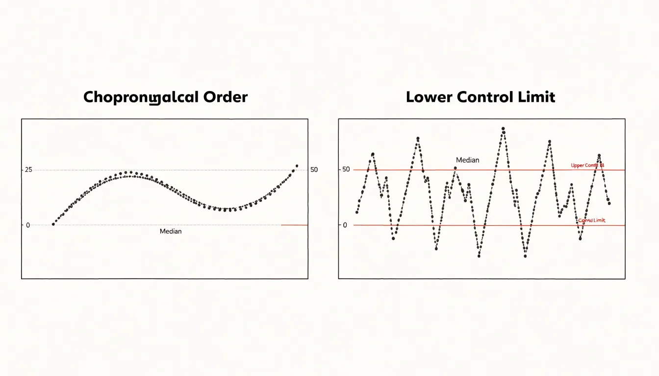
Run rules provide a structured way to interpret sequences of plotted points, catching subtle shifts before a point breaches a three-sigma limit. The Western Electric rules and the later Nelson rules define specific non-random configurations, such as seven or eight consecutive points on one side of the centerline, or six points steadily trending upward or downward.
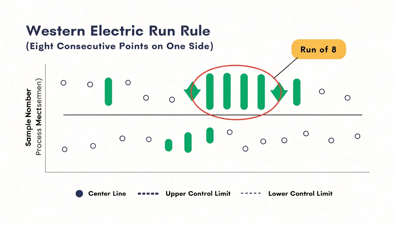
These pattern-based rules surface gradual changes early. A slow drift in a machine setting, gradual tool wear, or a creeping change in raw material characteristics often produces points that remain inside the control limits while forming a recognizable trend. Without run rules, such drift can continue undetected until the process pushes past a limit and generates a spike in defects. Watching for non-random arrangements gives quality teams advance warning while corrective action remains cheap and straightforward.
However, each additional rule increases both sensitivity to real shifts and the chance of false alarms. Practitioners should select rule sets suited to their specific process, verify signals before acting, train operators to read patterns consistently, and document responses to each signal.
Baseline Limits
Baseline limits are constructed from historical data to establish a reference period reflecting normal process behavior. A sufficient number of data points—typically 20 to 30 subgroups (or 20 to 25 for initial setup)—is recommended to capture the typical range of variation. This reference period must be free from known special causes, such as equipment failures, material shortages, or operator errors, so the calculated limits reflect only the inherent capability of the system.
When a process is in statistical control, baseline limits serve as a benchmark for future performance and a tool for forecasting operational yield. By quantifying expected variation, analysts can estimate the proportion of output that will fall within customer specification limits. This predictive capability supports setting realistic production targets and managing customer expectations.
Avoiding False Alarms
Preventing knee-jerk adjustments (tampering) when points fall within control limits requires discipline and structure:
- Train personnel: Ensure everyone who touches the process can distinguish between a single point inside the limits and a genuine out-of-control signal.
- Build explicit response procedures: Specify who may adjust the process and under what conditions, preventing informal fiddling during routine readings.
- Log rather than act: Encourage operators to record observations instead of adjusting immediately, creating a history that can be reviewed later for genuine patterns.
- Review at defined intervals: Checking charts on a schedule rather than continuously gives the process room to express its normal behavior.
- Reinforce restraint: Leadership should reward teams for holding steady when the data shows a stable process, reserving intervention for verified signals.
Recalibrating Boundaries
Recalibrating boundaries means updating the center line and control limits whenever a process has genuinely changed or improved, ensuring the chart reflects current rather than historical performance. When an improvement produces a sustained shift or a visible reduction in variation, existing limits become stale. Continuing to plot against them can make common-cause variation from the improved process appear as a string of out-of-control signals, while genuine new problems can hide behind limits that are now too wide.
Recalculation should follow evidence: wait until the change has demonstrated stability across 20 to 25 subgroups drawn from the new operating conditions. Analysts confirm the shift through standard chart signals, verify that the underlying causes are understood and documented, and only then recalculate the boundaries from the fresh data. Premature recalculation risks freezing limits around a temporary fluctuation, while indefinite delay anchors the chart to a process that no longer exists. Documenting the date, reason, and data window for each recalibration preserves traceability as baselines rise over time.
Common Tracking Mistakes
A handful of recurring data-handling mistakes can undermine otherwise sound control chart analysis:
- Miscalculating sample sizes: When subgroup sizes are inconsistent or incorrectly recorded, control limits no longer reflect true variation. An accidentally small subgroup inflates apparent variability, while an oversized one masks real shifts. Define subgroup size before collection begins, document it, and verify it whenever subgroups are combined or split.
- Plotting data out of order: Entering points out of chronological sequence scrambles the run patterns that signal special-cause variation. A single transposed date can create the illusion of a trend or hide a genuine shift. Use a consistent, timestamped data entry process and sort records by time before plotting.
- Ignoring early control signals: The first few out-of-limit points or unusual runs carry high diagnostic value, yet are sometimes dismissed as startup noise. Reviewing each new point as it arrives and treating early warnings as actionable prevents a drifting process from becoming costly.
Long Term Quality Control
Long-term quality control depends on embedding statistical process control into daily operations rather than applying it only during audits or troubleshooting. When charts are part of routine work, operators, supervisors, and managers share a common language for variation, capability, and stability, turning quality into a distributed capability that survives staff turnover and production cycles.
Sustaining this habit requires regular review meetings to discuss signals, training programs that pair statistical concepts with plant-floor examples, recognition for teams that resolve assignable causes, and documented procedures. Over time, this creates a feedback loop where measurement informs action and action generates new data, driving cumulative, incremental improvements rather than occasional large interventions.
Frequently Asked Questions
What should be recorded in a daily control chart log?
Operators should begin each shift by recording the same set of measures at the same time: extraction volume, temperature, pressure, and yield for every small batch. Each small batch should also be logged with its start time, duration, and output weight, plotted against the target band, and notes should be made when a batch falls outside expected limits.
What causes natural batch-to-batch variation in essential oil?
Natural batch-to-batch variation comes from biological factors such as plant genetics, age, and harvest stage, plus environmental conditions like sunlight, temperature, rainfall, soil, altitude, and harvest timing. The practical result is minor variation in aroma, viscosity, and chemical profile, meaning consistency is a matter of degree rather than an absolute.
What is common cause variation and should you adjust for it?
Common cause variation is the ordinary background noise of a process—the sum of many small, essentially random influences built into how the system operates. When only common cause variation is present, the appropriate response is to leave the process alone and, if improvement is desired, address the system as a whole rather than chase individual points.
What are examples of special cause variation and how should they be investigated?
Special cause variation appears as data points outside calculated control limits or as non-random patterns, and common examples include equipment malfunctions, raw material shifts, and environmental factors. Once flagged, investigate the root cause by checking equipment logs, reviewing material certificates, or interviewing operators.
How do you choose the right control chart for your data?
Continuous data call for variable charts such as X-bar and R, X-bar and S, or individuals and moving range (I-MR), while discrete data require attribute charts such as p or np for defectives and c or u for defects per unit.
When should control chart limits be recalculated?
Recalculate boundaries when a process has genuinely changed or improved and the change has demonstrated stability across 20 to 25 subgroups drawn from the new operating conditions. Confirm the shift through standard chart signals and verify that the underlying causes are understood and documented before recalculating.
Tony Astor
Tony writes about data visualization and the tools people use to build charts and dashboards. More about Data Illustrator