Choropleth Map: How to Map Data by Region
 By Tony Astor ·
Choropleth Map
A choropleth map is a thematic map that shades predefined geographic regions—countries, states, counties, or census tracts—in proportion to a data value for each region, with colors matched to a legend. It suits aggregated data such as population density, election results, or disease rates, and works best with rates or ratios rather than raw counts.
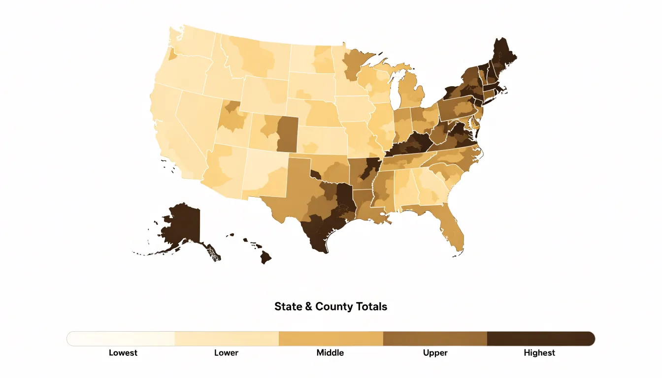
Table of Contents
Choropleth Map
A choropleth map is a thematic map in which predefined geographic regions—such as countries, states, counties, or census tracts—are shaded or patterned in proportion to a data value associated with each region. The name derives from the Greek words choros (region) and plethos (multitude), and the form is one of the oldest and most widely recognized conventions in thematic cartography. Each region receives a fill color or pattern drawn from an ordered visual scale, and the reader decodes the underlying value by matching that fill to a legend. Because the geography itself supplies the shapes, the map functions as a kind of spatial bar chart, letting viewers compare magnitudes across many places at once while preserving the familiar outlines of the territory.
Choropleth maps are at their strongest when the data are already aggregated to administrative or statistical units and when the phenomenon varies meaningfully from one region to another. Population density is a classic case: residents per square kilometer, computed for each county or district, translate naturally into a graduated shading scheme that reveals urban cores, suburban fringes, and sparsely settled hinterlands in a single glance. Election results offer another ideal fit, since votes are tallied by precinct, district, or state and the share won by a candidate can be mapped directly onto those boundaries, producing the familiar red-and-blue renderings that dominate political coverage. Other suitable applications include rates of disease incidence by health district, median household income by census tract, literacy levels by province, and crime counts by police sector.
The technique works best when regions are of roughly comparable size, when the variable is a rate or ratio rather than a raw count, and when the number of classes is kept modest so the legend remains readable. Under those conditions, regional shading transforms a table of numbers into an immediate visual statement about how a phenomenon is distributed across space.
Choropleth Map
Raw counts often mislead viewers because they conflate population size with the underlying phenomenon. A region with more people will naturally have more cases, sales, or incidents, even if the per-person risk is identical to a smaller region. When a choropleth map shades regions by raw totals, large population centers dominate the visual field, drawing attention away from smaller areas that may have higher rates. This distortion can lead viewers to infer that densely populated areas are always worse off, when in fact the map is simply reflecting population distribution rather than the intensity of the topic being mapped.
To ensure accurate spatial comparisons, analysts should convert raw counts into rates, percentages, or per-capita metrics:
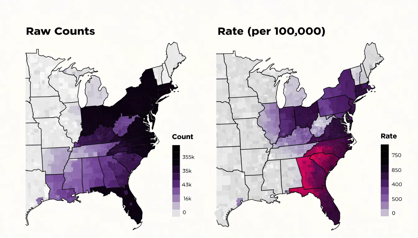
- Rates, such as cases per 100,000 people, adjust for population size and allow direct comparison across regions of different sizes.
- Percentages work well for part-to-whole relationships, like the share of households with broadband access.
- Per-capita metrics, such as income per person or spending per resident, provide a normalized basis for comparing economic or service-related data.
The choice among these depends on the nature of the data and the question being asked, but the goal remains the same: to remove the influence of population size so that the map reveals patterns in the underlying phenomenon.
Normalization also helps mitigate the visual dominance of large regions. When rates are mapped, small areas with high rates can stand out just as clearly as large areas with high rates, leading to a more balanced and truthful representation. Additionally, normalizing data can reduce the impact of outliers and make the map more robust to variations in reporting or data collection.
Choropleth Map
The choice of geographic aggregation level is one of the most consequential decisions in building a choropleth map, because the boundaries drawn around the data determine what patterns become visible. Data aggregated by zip code, county, or state will tell noticeably different stories even when the underlying observations are identical. A state-level map smooths variation across large populations into a single color, which can hide sharp disparities between urban cores and rural areas. A county-level map recovers much of that variation, while a zip-code map pushes the resolution further and exposes neighborhood-scale contrasts that coarser units flatten out.
This sensitivity is often described through the modifiable areal unit problem, which captures the fact that statistical results shift when the same data are grouped into different sets of zones. Boundaries are rarely neutral; they follow administrative histories, political decisions, and population distributions that may have little to do with the phenomenon being mapped. As a rule, smaller units preserve more local detail and allow finer distinctions, though they also introduce more visual noise and smaller denominators that can produce unstable rates. Larger units offer stability and cleaner visual summaries at the cost of concealing heterogeneity within each region.
The selection also interacts with map perception. Readers intuitively associate the area of a region with its importance, so large rural counties or states can dominate the visual impression even when they contain relatively few people. Maps built on small, densely packed urban units can appear fragmented and hard to compare. Choosing boundaries therefore involves balancing analytical resolution, statistical reliability, and legibility. Practitioners typically begin with the analytical question, select the finest unit that still yields dependable estimates, and disclose the aggregation level alongside the map so readers understand what the pattern represents and what it necessarily obscures.
Choropleth Map
Data classification is the process of deciding how the full range of observed values should be divided into a manageable number of groups, each of which receives a single color or shade. When a dataset contains hundreds or thousands of distinct values—such as population density, median income, or unemployment rates—a map that assigned a unique color to every value would be impossible to read. Binning those continuous values into a small number of classes solves this problem by reducing visual complexity while preserving the overall geographic pattern.
The classification step begins with an examination of the data’s distribution, including its minimum, maximum, and the way values cluster or spread across the range. Analysts then choose a method for placing class breaks, the boundary values that separate one bin from the next. Common approaches include equal intervals, quantiles, natural breaks, and custom thresholds tied to meaningful benchmarks. Each method produces a different set of breaks and therefore a different map, even when the underlying numbers stay the same.
The number of classes also matters. Too few bins flatten important variation, while too many overwhelm the reader and make legends hard to interpret. Most choropleths use between four and seven classes, a range that keeps the legend legible and the shading distinguishable.
Choropleth Map
Because the classification method determines which regions appear dark and which appear light, two of the most common approaches—equal interval and quantile classification—divide ranges in fundamentally different ways.
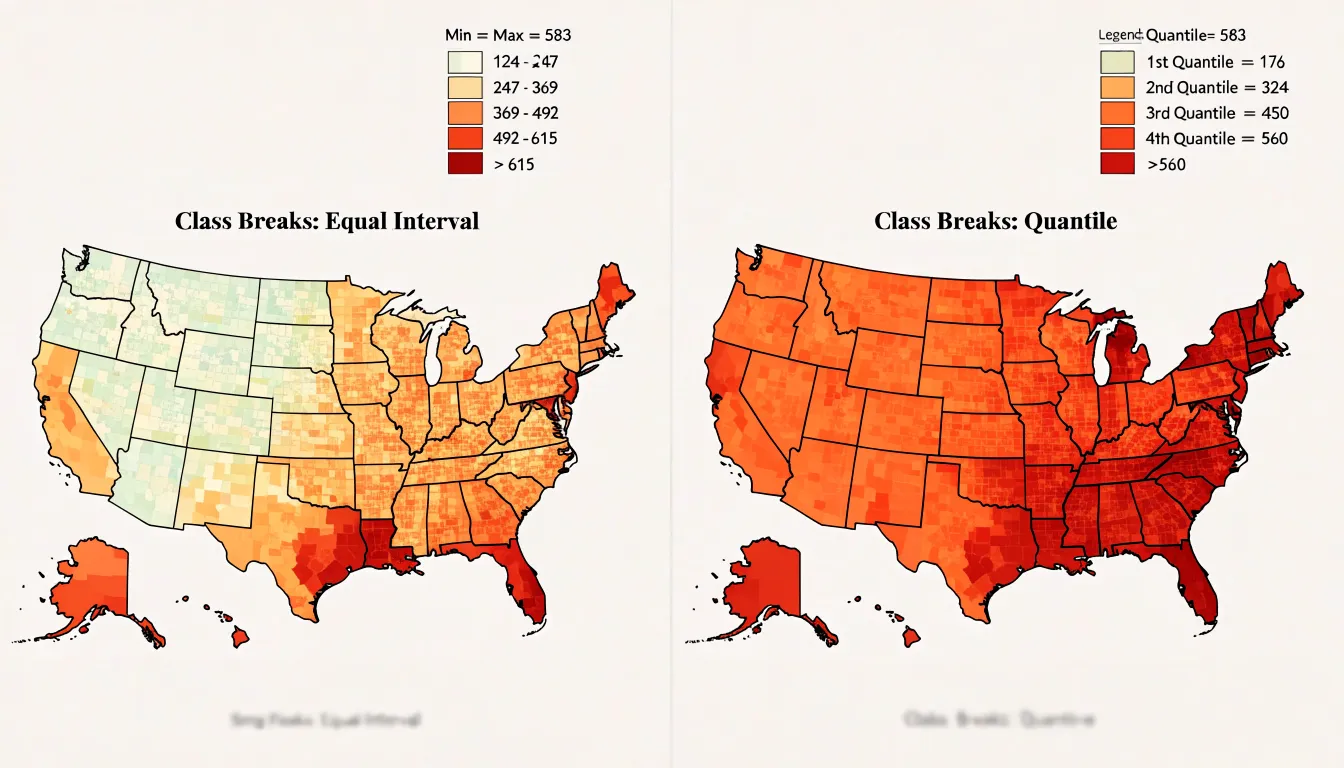
Equal interval classification takes the full range of values, from the minimum to the maximum, and splits it into a set number of bins of identical width. If values run from 0 to 100 and five classes are requested, each class spans 20 units. The appeal of this method is that the legend is easy to read and interpret: each color step represents the same amount of change in the underlying variable. This makes equal interval well suited to data that are evenly distributed or to variables where absolute differences matter, such as rates per capita or percentages where readers care about equal increments on a scale.
Quantile classification works differently. Instead of dividing the value range evenly, it places an equal number of observations, such as counties or census tracts, into each class. With five quantiles and 500 observations, each class holds roughly 100 observations. The boundaries between classes therefore fall at very different value points, and some classes may cover wide value ranges while others cover narrow ones. This approach is useful when the data are heavily skewed or clustered, because it guarantees visual variation across the map and prevents most areas from falling into a single class.
The trade-off is that quantile classes can group dissimilar values together and make modest differences look dramatic, while equal interval classes may produce a map dominated by one color if the data contain extreme outliers. In practice, the choice depends on the shape of the data and the story the map should tell: equal interval for straightforward, absolute comparisons, and quantile when the goal is to reveal relative rankings and ensure each class is represented.
Choropleth Map
The Jenks natural breaks algorithm is a data classification method that seeks to partition a dataset into groups that are internally homogeneous and externally distinct. It works by minimizing the variance within each class and maximizing the variance between classes, effectively identifying natural groupings inherent in the data without imposing an arbitrary classification scheme.
The algorithm operates iteratively: it considers all possible ways to divide the sorted data into a given number of classes and selects the arrangement that minimizes the sum of squared deviations from each class mean. In practice, this means that boundaries are placed where there are relatively large gaps between data values, so that each class contains values that are similar to one another. The result is a set of classes that reflect the actual distribution of the data, rather than forcing it into equal intervals or quantiles.
For choropleth mapping, natural breaks can be advantageous because they highlight clusters and outliers that might be obscured by other methods. For example, if a variable such as population density has a few extremely high values and many moderate values, natural breaks will create a separate class for the high outliers, preventing them from skewing the color scale. This makes the map more informative and easier to interpret, as the visual differences correspond to meaningful breaks in the data.
However, natural breaks are not without drawbacks. The method is data-driven, so the class breaks can change if the underlying data changes, making comparisons across maps or over time difficult. Additionally, the algorithm can be computationally intensive for large datasets. Despite these limitations, Jenks natural breaks remain a popular choice when the goal is to reveal the inherent structure of the data and to minimize within-group variance.
Choropleth Map
Choosing a sequential color scheme for a choropleth map begins with the recognition that the colors themselves carry meaning before any legend is read. A sequential scheme should progress in a smooth, ordered way from light to dark or from low saturation to high saturation, so that a reader glancing at the map immediately senses direction and magnitude. Single-hue gradients, such as a pale yellow rising through amber to deep brown, are often the safest choice because varying lightness along one hue produces a natural sense of increase. Multi-hue gradients can work equally well when they follow a perceptually ordered path, for example moving from light green through yellow to dark blue or purple, as long as each step remains clearly distinguishable from its neighbors.
The central concern is that the visual progression matches the numeric progression. Human vision interprets darker and more saturated colors as heavier or more intense, so the darkest end of the ramp should correspond to the highest values and the lightest end to the lowest. Reversing that relationship, or introducing a hue that appears artificially bright in the middle of a scale, can lead readers to misread the data. Designers should also consider whether the variable is naturally ordered from low to high, since sequential schemes assume a continuous, monotonic relationship between color and value.
Perceptual uniformity matters greatly here. Some gradients compress adjacent categories so tightly that readers cannot separate them, while others leap between steps too dramatically. Testing the ramp in grayscale reveals whether lightness alone carries enough information, and checking colorblind simulations guards against confusion between hues.
Choropleth Map
A diverging color scheme is a valuable choice when a choropleth map is intended to reveal how regions deviate from a meaningful midpoint. The defining feature of this palette is a neutral hue at the center that transitions into two distinct color families moving outward in opposite directions. Common examples place a pale gray or soft cream at the middle, with shades of blue intensifying toward one end and shades of red or orange intensifying toward the other. The visual result separates values above the midpoint from values below it while keeping the midpoint itself visually quiet.
This structure works best when the midpoint carries real analytical meaning. A national average is a frequent anchor: states or counties scoring above the country-wide rate take on one hue, and those below it take on the complementary hue. A zero-change baseline serves the same purpose in maps tracking year-over-year shifts, where positive growth and decline are equally important to display. Diverging palettes also suit temperature anomalies, budget surpluses and deficits, and any measurement where the direction of departure matters as much as its size.
The dual palette encodes direction through hue and magnitude through saturation. As values move further from the midpoint, colors grow darker or more intense, so extreme cases stand out immediately. The faint center keeps average regions in the background and lets the viewer scan for outliers without reading every legend entry.
Designers should choose the two arms so that neither appears more prominent than the other, since equal visual weight prevents one side of the scale from dominating the reader’s impression. A clear legend with the midpoint labeled, and symmetric class breaks on either side, helps the audience interpret the map accurately and compare deviations across the whole geography.
Choropleth Map
Designing a clear legend begins with the structure of the scale markers themselves. Whether the map uses discrete class breaks or a continuous gradient, the legend should present the markers in a consistent spatial order, typically running from lowest to highest value along a horizontal bar or a vertical stack. Each marker should occupy an equal visual footprint so that the intervals read as a coherent sequence rather than an irregular patchwork. When class breaks are uneven, the legend spacing can remain uniform while the accompanying labels explain the actual numeric boundaries.
Labels sit at the heart of legend legibility. Each color block or gradient stop should carry a concise label showing the range it represents, using consistent formatting for numbers, units, and decimal precision. Round values where possible, and place labels so they align with the boundaries between blocks rather than floating ambiguously inside them. A short title above the legend identifies the variable being mapped, while a brief note can clarify the data source, year, or classification method.
Color blocks themselves deserve deliberate treatment. Adjacent classes should differ enough in hue or lightness that readers can distinguish them at a glance, and the ordering should follow an intuitive progression from light to dark or cool to warm. Including a subtle border around each block helps separate neighboring shades. Testing the legend with a few viewers and refining spacing, label length, and color contrast will reveal where confusion arises before the map reaches a wider audience.
Choropleth Map
A few recurring color mistakes can quietly undermine an entire choropleth map:
- The rainbow palette: Mapping values onto a spectrum that runs through green, yellow, and red creates artificial boundaries where hue shifts abruptly, so viewers perceive sharp breaks in the data that do not exist. Rainbow schemes also lack a natural perceptual order; some hues appear brighter or more saturated than others regardless of the underlying value, which leads readers to rank regions by color intensity rather than by the actual numbers. Instead, use sequential or diverging palettes as appropriate for the data.
- Insufficient value contrast: When adjacent classes in a legend are too similar in lightness, readers cannot reliably distinguish one region from another, particularly on smaller screens or in print. Setting the class breaks so that each step differs noticeably in value, and testing the result in grayscale, helps confirm that the pattern survives without relying on hue alone.
Choropleth Map
Choropleth maps depend on a clean join between thematic data and geographic boundaries, and two persistent problems can undermine that join: extreme values that distort the visual story, and shapefiles whose boundaries do not align with the data’s reporting units.
Working with outliers starts with inspection. Plotting the value distribution as a histogram or ranking the units by value reveals whether a handful of observations sit far above the rest, as often happens with population counts or economic totals in large metropolitan areas. Several strategies can reduce the distortion these values create:
- A logarithmic or square-root scale compresses the upper tail so that mid-range variation remains visible.
- Quantile breaks are less sensitive to high extremes than equal-interval schemes, while a manually capped maximum, with an explicit note in the legend, keeps a single outlier from washing out every other color.
- Robust statistics such as the median and interquartile range provide alternative anchors when setting breakpoints.
- Where the extreme values reflect a genuine phenomenon, reporting them in a separate category or an accompanying table preserves the information without letting it dominate the map.
Boundary mismatches arise when the geographic units in a shapefile differ from the reporting units in the dataset, for example when data arrive at postal code level but boundaries are drawn for census tracts. A crosswalk table that maps codes between the two systems is the standard remedy, and areal interpolation can estimate values for overlapping zones when no official correspondence exists. Before joining, checking that codes share a format, match on type, and cover the same geographic extent prevents silent losses. An analysis of unmatched records after the join shows whether gaps are minor or systematic, and units with no data should be shown distinctly as missing rather than colored as zero. Documenting these decisions keeps the map honest and reproducible.
Choropleth Map
Mapmakers carry a responsibility to ensure that the information encoded in color reaches every reader, including the roughly one in twelve men and one in two hundred women who experience some form of color vision deficiency. The most common forms, deuteranopia and protanopia, collapse distinctions between reds and greens, so a scheme that looks vivid and clearly graded to a designer may appear as an undifferentiated wash of similar browns to a substantial portion of the audience.
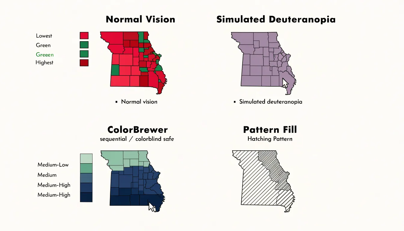
The practical answer begins with selecting palettes that have been tested against simulations of these deficiencies. ColorBrewer, developed by Cynthia Brewer, offers sequential, diverging, and qualitative schemes explicitly flagged as colorblind-safe, and its sequential palettes typically move through variations in lightness as well as hue, giving readers a redundant cue that survives the loss of one color channel. Tools such as Viridis and Cividis extend the same principle into continuous scales designed for perceptual uniformity.
Color choice alone does not guarantee universal access, however, and designers can strengthen a map further by varying texture alongside hue. Pattern fills, hatching at different angles, dots, and cross-hatching allow adjacent classes to be distinguished even when their colors appear identical. These textures function as a second encoding channel, so a reader who cannot separate two shades on the legend can still match a region to its class through the fill pattern. Care is needed to keep patterns subtle enough that they do not obscure the underlying geography or create visual noise, especially in maps with many small polygons. Combining tested palettes with strategic textures, clear legends, and optional data labels produces maps that communicate reliably to colorblind and color-typical readers alike.
Choropleth Map
Mobile screens impose tight constraints on choropleth maps, where detailed boundaries and dense legends can quickly overwhelm a small viewport. Responsive mapping techniques begin with fluid layout principles: the map container should scale to the device width, with vector tiles and adaptive projections that redraw cleanly at any size. Media queries can adjust legend placement, collapse supplementary controls into menus, and reposition labels so the core data story remains legible on a phone held in portrait orientation.
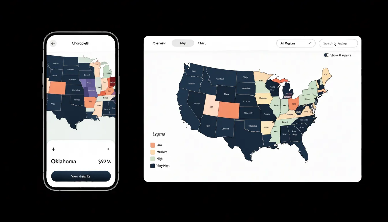
Simplified boundaries play an equally important role. Detailed polygon geometries that look crisp on a desktop monitor become visual noise at mobile scale, so cartographers generalize shapes using techniques such as Douglas-Peucker simplification, smoothing coastlines and administrative borders to a level appropriate for the display resolution. Topology-preserving simplification avoids slivers and gaps between adjacent regions, keeping the map visually coherent while reducing file size and rendering load.
Touch-friendly tooltips complete the mobile experience. Hover interactions have no equivalent on a touchscreen, so tooltips should trigger on tap and remain visible until the user taps elsewhere or closes them. Hit targets need to be large enough to accommodate a fingertip, which often means enlarging small polygons or providing a bottom sheet that displays the selected region’s values rather than relying on precise point selection. Placement matters too, with tooltips positioned to avoid covering the tapped area or extending beyond the screen edge.
Choropleth Map
Exporting clean graphics from a choropleth map starts with planning the output format around its final destination. For printed reports, vector formats such as SVG or PDF preserve crisp boundaries and text at any scale, so the map remains legible whether it appears in a narrow column or across a full page. Raster formats like PNG suit online publication and slide decks, where a fixed pixel dimension is often sufficient and file size matters. Setting the export resolution deliberately, typically at two to three times the intended display size for raster output, ensures that labels and thin boundary lines stay sharp on high-density screens and in print. Embedding or outlining fonts before export prevents text from shifting or falling back to substitute typefaces on another machine.
Layer hygiene contributes as much to clean output as resolution settings. Turning off extraneous gridlines, selection halos, and editor artifacts keeps the graphic focused on the data. A well-designed legend, scale bar, and source note travel with the map and should be positioned within the export bounds rather than left floating outside the canvas. Consistent color reproduction across formats depends on choosing a color mode that matches the medium: RGB for screen, CMYK for professional printing, with the palette checked after conversion since vivid hues can shift noticeably.
File organization and naming also support professional workflows. Descriptive file names that include the map subject, date, and format version make assets easy to locate and update later. Where the map will be reused, exporting a layered or editable master alongside the final flattened graphic saves time when data changes. Checking the exported file at its actual display size, zooming in on dense areas and small labels, catches problems that remain invisible in the editor.
Choropleth Map
Creating effective choropleth maps depends on selecting software that matches both the technical skills of the mapmaker and the intended audience. Desktop GIS platforms such as QGIS and ArcGIS Pro offer comprehensive environments for data classification, projection handling, and cartographic design, and they suit analysts who need to prepare static or print-oriented maps with careful attention to legend and colour choices. For web-based delivery, JavaScript libraries such as Leaflet, D3.js, Mapbox GL JS, and Plotly provide a range of approaches, from lightweight tile-based rendering to fine-grained control over SVG geometry and transitions. Each option carries trade-offs in learning curve, performance with large datasets, and the degree of customisation available for styling polygons according to data values.
Interactive features often distinguish a web-based choropleth map from a static graphic:
- Hover effects give users immediate feedback by revealing the name of a region and its underlying value, frequently through tooltip overlays or highlighting the polygon beneath the cursor.
- Click interactions can open detail panels, navigate to related views, or trigger updates in linked charts.
- Filtering controls let viewers narrow the data by category, time period, or threshold, which helps when a single map would otherwise combine too many variables.
- Slider controls support temporal exploration, while dropdown menus and checkboxes allow users to switch between datasets or isolate specific regions.
- Zoom and pan behaviour, combined with appropriate scale-dependent styling, helps maintain legibility across different geographic extents.
For web accessibility and performance, interactive elements should be reachable via keyboard where possible, and using canvas rendering alongside simplified geometry and vector tiles can keep large polygon datasets responsive during hover and filter operations.
Frequently Asked Questions
What is a choropleth map?
A choropleth map is a thematic map in which predefined geographic regions are shaded or patterned in proportion to a data value associated with each region. Readers decode the underlying value by matching each region’s fill to a legend.
Why are raw counts misleading in choropleth maps?
Raw counts can conflate population size with the underlying phenomenon, so large population centers dominate the visual field. To compare regions accurately, analysts should convert raw counts into rates, percentages, or per-capita metrics.
How does the choice of geographic aggregation level affect a choropleth map?
Data aggregated by zip code, county, or state can tell noticeably different stories even when the underlying observations are identical. Smaller units preserve more local detail but can introduce visual noise and unstable rates, while larger units offer stability but conceal heterogeneity within each region.
What is the difference between equal interval and quantile classification?
Equal interval classification splits the full range of values into bins of identical width, while quantile classification places an equal number of observations into each class. Equal interval is suited to straightforward absolute comparisons, while quantile is useful when data are heavily skewed or clustered and the goal is to reveal relative rankings.
What are the drawbacks of Jenks natural breaks?
Jenks natural breaks are data-driven, so the class breaks can change if the underlying data changes, making comparisons across maps or over time difficult. The algorithm can also be computationally intensive for large datasets.
How can I make a choropleth map accessible to colorblind readers?
Use palettes tested against simulations of color vision deficiency, such as ColorBrewer schemes explicitly flagged as colorblind-safe, plus tools like Viridis and Cividis. Designers can also vary texture alongside hue using pattern fills, hatching, dots, and cross-hatching, while keeping patterns subtle enough not to obscure geography or create visual noise.
Tony Astor
Tony writes about data visualization and the tools people use to build charts and dashboards. More about Data Illustrator