Chart Axis Best Practices: Scales, Ticks and Gridlines
 By Tony Astor ·

Chart Axis Best Practices
Bar charts and area charts must start their value axis at zero, because bar length encodes magnitude and a truncated baseline exaggerates small differences into large visual gaps. Line charts may use a non-zero baseline for large-magnitude time series, provided the axis minimum is clearly labeled.
Table of Contents
- Zero Baseline Rules
- Truncated Axis Risks
- Linear Scale Applications
- Logarithmic Scale Basics
- Dual Axis Pitfalls
- Tick Mark Placement
- Major vs Minor Ticks
- Number Formatting Tips
- Label Rotation Guide
- Gridline Density Rules
- Time Series Axis Layouts
- Categorical Axis Setup
- Aspect Ratio Essentials
- Accessibility Axis Standards
Zero Baseline Rules
Bar charts encode value through the length of each bar, measured from the axis baseline. When the baseline sits at zero, every bar’s length is directly proportional to the quantity it represents, so a value twice as large produces a bar twice as long. This proportionality is the entire basis for reading a bar chart accurately. Moving the baseline upward breaks that relationship, because the visible portion of each bar no longer reflects the full magnitude of the underlying number. A small difference between two values can then appear as a large visual gap, and readers who scan the chart without checking the axis labels will draw conclusions the data does not support.
Consider two categories measuring 102 and 104 units. On a zero-based axis, their bars differ by roughly two percent, and the visual impression matches the modest real difference. If the axis starts at 100 instead, the bars render as lengths of 2 and 4, and the second appears twice as tall as the first. The chart now communicates a dramatic gap where the underlying numbers show near parity. This kind of distortion is easy to produce accidentally, since many charting tools will auto-scale to the data range by default, and the resulting graphic can look polished while quietly misrepresenting the data.
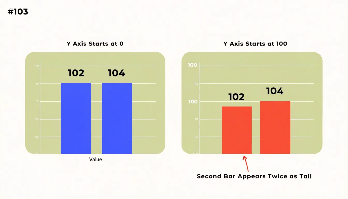
A zero baseline is therefore required for any chart that encodes magnitude through length or area, including stacked and grouped bar charts, histograms, and area charts. When the variation in a dataset is genuinely small and detail matters, the appropriate solution is a chart form built for that purpose, such as a line chart with a clearly labelled non-zero axis or a dot plot, rather than a bar chart with a truncated scale. Keeping bars anchored at zero preserves the reader’s ability to compare lengths honestly.
Truncated Axis Risks
Truncated axes appear frequently in business reporting because they make small changes look dramatic. A bar chart starting its y-axis at 95 instead of zero can turn a two-percent revenue shift into a visual cliff. A company comparing quarterly earnings across divisions can make one unit appear to be collapsing while another seems to have doubled, even when both moved by a fraction of a percent. Political coverage has faced similar criticism, where polling charts with compressed scales suggest wild swings in public opinion that the underlying data does not support. In each case, readers absorb the visual slope before they read the numbers.
The ethical challenge is that legitimate small changes often deserve attention. A half-point gain in customer retention or a one-percent drop in error rates can matter enormously for a product team. The goal is to surface those movements without implying they are larger than they are. While bar charts must anchor at zero, line charts encode change in position and can use a non-zero baseline when starting at zero is impractical for large-magnitude time series. Designers can clearly label the axis minimum, state the reason for the range, add a break symbol, and pair the trend line with a direct annotation of the actual values. Dual encoding also works well: show the change as a labeled number alongside a sparkline whose scale is disclosed.
Contextual cues also matter. Annotations noting the absolute difference, comparison benchmarks, and uncertainty ranges give readers the grounding to interpret modest movements correctly. Designers who document scale decisions and test charts with colleagues can catch unintended narratives. Readers should always be able to see where the axis begins and judge the size of any change for themselves.
Linear Scale Applications
Linear scales assign equal visual spacing to equal numeric intervals, so a difference of ten units occupies the same distance anywhere along the axis. This consistency lets readers translate position into value almost automatically, without mental arithmetic. For continuous variables such as revenue, session duration, temperature, distance, or time elapsed, equal-interval spacing matches how people already reason about quantity.
Standard business metrics are especially well served by this default. Monthly sales totals, website traffic, average order values, headcount, and customer counts all behave as continuous quantities measured on a regular interval. With uniform spacing, a line rising at a steady slope signals steady growth. These readings feel immediate in a dashboard or report.
The sensible approach in most situations is to begin with a linear scale and depart from it only for a specific, documented reason. Equal-interval spacing keeps comparisons fair across the whole range of the axis, avoids exaggerating small changes near one end, and makes annotation, reference lines, and target markers easy to place and interpret. Analysts and executives alike read it without explanation.
To support intuitive reading, anchor bar and area axes at zero, choose tick intervals that divide evenly (steps of 5, 10, 25, or 100), and label enough gridlines for orientation without crowding the plot.
Logarithmic Scale Basics
Logarithmic scales display data that spans several orders of magnitude. On a linear axis, a dataset that grows from 10 to 10,000 leaves the earliest values clustered so tightly near the baseline that they become impossible to distinguish. A logarithmic axis solves this by spacing values according to their order of magnitude: equal distances correspond to equal multiplicative factors, such as doubling or a tenfold increase. A value of 100 sits midway between 10 and 1,000 in visual terms, even though its absolute distance from each endpoint differs enormously.
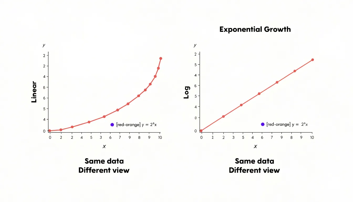
This compression is especially valuable for exponential growth. Viral adoption curves, compound interest trajectories, and economic expansion over long horizons often share a shape where early growth is dwarfed by later totals. Plotted linearly, the early phase collapses into a flat line hugging the axis, while the final values dominate the chart. With a logarithmic scale, each successive period of exponential growth appears as a consistent upward slope, revealing whether the rate of change is steady, accelerating, or decelerating. A straight line on a log axis indicates constant percentage growth, making deviations immediately visible.
Log scales also allow comparing series with vastly different magnitudes on a single chart without one overwhelming the others. When preparing such a chart, label the axis with the actual values at major tick marks rather than the exponents, and consider noting that the scale is logarithmic in the axis title. Readers unfamiliar with log scales can misread visual distance as proportional to absolute difference, so clear labeling preserves interpretability.
Dual Axis Pitfalls
Dual y-axes introduce perceptual traps that even experienced analysts can fall into. When two metrics share a chart with separate vertical scales, the eye naturally reads the crossing and divergence of the lines as meaningful events. In reality, the intersection point is determined almost entirely by arbitrary scale choices, not by any relationship in the underlying data. Shift one axis’s minimum or maximum and the crossover point slides along the x-axis without a single data value changing. Readers rarely pause to check which line belongs to which axis, and color alone is a fragile cue when lines are close together. The result invites confident but incorrect conclusions about correlation, timing, and causation.
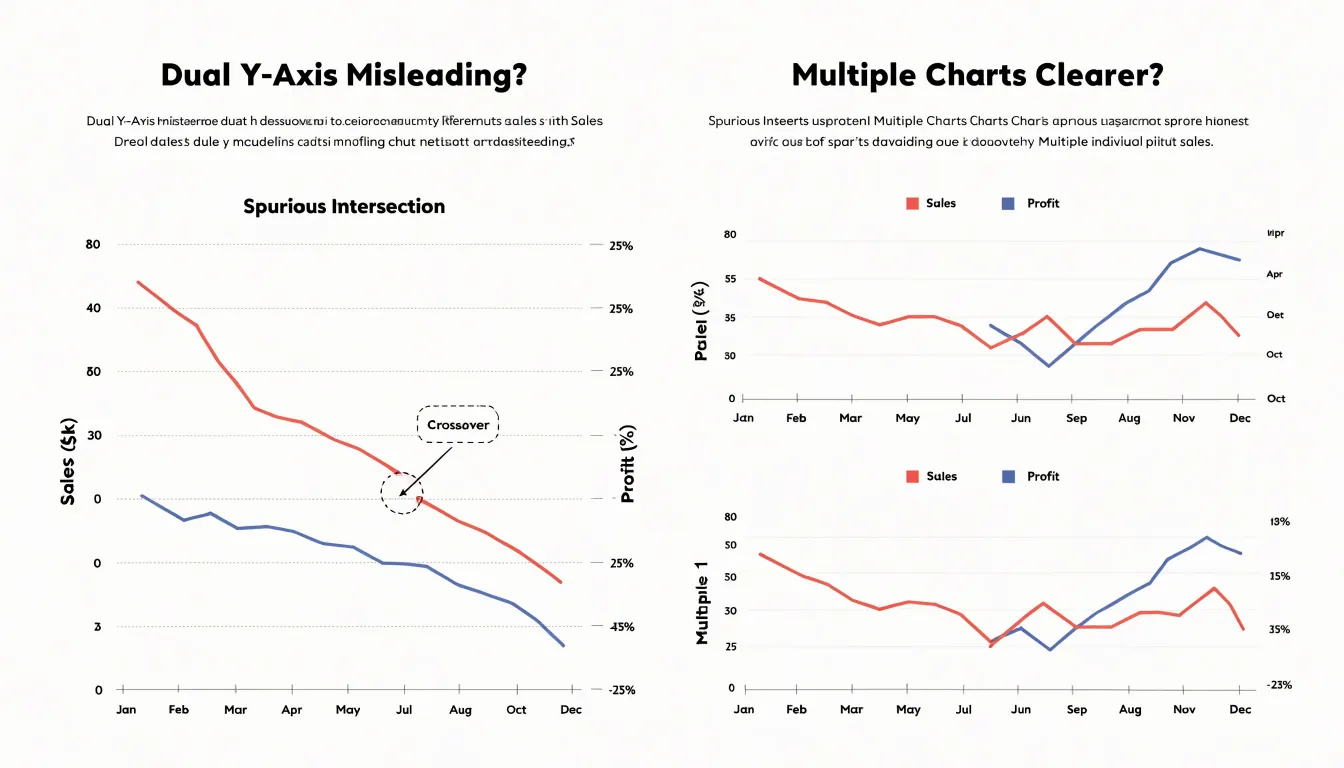
Mismatched scales amplify the problem. A metric spanning thousands paired with one spanning single digits forces one series to hug the baseline while the other swings dramatically, visually implying volatility where none exists. Changing the axis range can manufacture a dramatic trend or flatten a genuine one, and because both series look equally authoritative, viewers have no way to judge which visual impression reflects the data. Truncated axes and logarithmic scaling on only one side compound the ambiguity.
Small multiples offer a cleaner path. Placing each metric in its own panel with a shared x-axis lets readers compare trends across aligned time periods without implying that the lines interact. Each panel gets an honest scale, and the eye can track patterns across panels without being seduced by spurious intersections. Where a combined view is genuinely needed, consider indexing both series to a common baseline so a shared axis becomes meaningful. Annotating axes clearly and labeling series directly beside their lines helps when a dual axis is unavoidable, but small multiples or indexed values usually communicate the comparison with far less risk of misreading.
Tick Mark Placement
Tick mark placement is an arithmetic challenge: the axis must span the full numeric range of the data, yet the viewable area places a hard ceiling on how many labels can sit along that span without colliding. Begin by measuring the actual length of the axis in pixels, then divide by the minimum space a single label requires. A short numeric label such as “40” might need roughly 30 to 40 pixels of horizontal room, while a date label like “Mar 2025” needs considerably more. The resulting quotient gives the maximum number of ticks the axis can hold while remaining legible.
With that ceiling in hand, subtract the minimum value from the maximum to get the numeric span, then divide by the maximum tick count to find a rough interval size. Raw intervals rarely produce pleasant labels, so round the result up to a friendly value: steps of 1, 2, 5, or 10 multiplied by a power of ten, or calendar-aligned units such as weeks, months, or quarters for time series. This rounding usually reduces the tick count slightly below the ceiling, adding breathing room between labels.
Next, verify the generated labels. Check the first and last ticks against the axis bounds to confirm they fall inside the viewable area and do not clip against the chart edges. Confirm that no two labels overlap at the smallest expected rendering size, since responsive layouts may shrink the axis. When the computed interval would still produce crowding, drop to the next larger friendly step rather than shrinking the font, or abbreviate large ranges, preserving readability across devices and viewing distances.
Major vs Minor Ticks
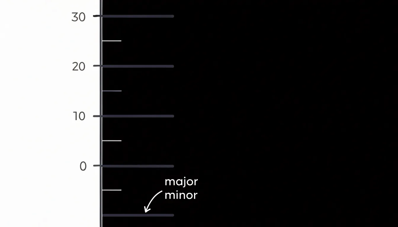
Major tick marks anchor the axis with labeled values at regular, meaningful intervals, such as increments of ten on a range from zero to one hundred. Because major ticks carry labels, they form the backbone of the axis and should receive the strongest visual treatment, typically a slightly longer line and a label set in legible type. Consistent interval spacing helps readers estimate intermediate values by eye and keeps the chart predictable across multiple axes.
Minor tick marks sit between the major ticks and divide each interval into smaller units to help readers estimate intermediate positions without adding more text. Their usefulness depends on restraint. A single subdivision between each pair of major ticks can aid estimation, whereas too many crowd the axis line and compete with major ticks for attention. Minor ticks should therefore be shorter and lighter in weight than major ticks, often rendered in a muted gray, and left unlabeled to preserve the visual hierarchy. In dense or small-format charts, removing minor ticks entirely is often the better choice. Major ticks should carry the interpretive weight, with minor ticks appearing only where they measurably improve reading accuracy.
Number Formatting Tips
When every tick carries six or seven digits, the reader has to count zeros to grasp the magnitude, and the axis becomes a dense wall of numerals that competes with the data. Abbreviating numbers with standard scale indicators resolves this simply. Values in the thousands become ‘K’, millions become ‘M’, and billions become ‘B’, turning 45000000 into a compact 45M. Readers already recognize these suffixes from financial reports, social media metrics, and dashboard tools. Place the scale indicator in a consistent position across every tick, and state the unit once in the axis title or a small corner note so the meaning stays unambiguous.
Currency values benefit from the same discipline. Symbols such as ’$’ or ’€’ can appear once in the axis title rather than on every individual tick, and decimal places should match the precision the data actually supports. Showing cents on a revenue axis measured in millions adds noise without information. For percentage axes, pick a single decimal convention, apply it uniformly, and avoid mixing raw proportions like 0.25 with formatted percentages like 25% on the same scale. Consistent abbreviation, restrained decimals, and a single declared unit keep labels scannable.
Label Rotation Guide
Angled axis labels force readers to tilt their heads or trace diagonals with their eyes. Research on reading behavior shows that people recognize rotated words significantly more slowly than horizontal ones, with each additional degree of tilt adding measurable cognitive cost. In a chart, that cost compounds across every label on the axis. Treat rotation as a last resort and redesign the chart so labels can stay horizontal.
The simplest fix is often switching chart orientation: when category names are long, a horizontal bar chart places those names along the vertical axis where they read left to right naturally. This eliminates rotation, preserves full label text, and frequently improves comparison accuracy, since horizontally aligned bars are easy to rank by length.
When a vertical layout is required, several alternatives keep text horizontal:
- Truncate strategically: Cap each label at a fixed character count, append an ellipsis, and provide the full text through a tooltip, legend, or accompanying table.
- Wrap text: Break long labels onto two or three lines at natural word breaks.
- Abbreviate: Use shortened category codes when the audience already knows them.
- Reduce label density: Show every other tick, or group minor categories under an ‘Other’ bucket to give remaining labels room to sit flat.
Gridline Density Rules
Gridlines help readers connect data marks to axis values, and their usefulness depends on their spacing and visual weight. When spaced too far apart, estimating a value between two reference lines requires guessing over a wide gap, introducing error. When spaced too closely, the plot area fills with lines that compete with the data itself. The goal is a density that provides a reliable anchor near any point while keeping the data visually dominant.
Target roughly four to seven gridlines across the full axis range, placed at intervals that match mental arithmetic—such as 1, 2, 5, 10, 20, 25, or 50—rather than awkward steps like 3, 7, or 13. On time axes, follow familiar calendar units (days, weeks, months, or years) rather than arbitrary day counts. Place axis labels at the same intervals so each reference line has an explicit value attached.
Gridlines should sit clearly behind the data marks, rendered in a light neutral tone such as pale gray that remains visible against the background but recedes at a glance. Thin strokes, often a single pixel, keep the lines from thickening the plot area visually. Solid lines generally work well at low contrast, though dashed or dotted styles can further reduce visual weight. If minor gridlines are included, make them lighter still, or omit them if major lines provide adequate anchoring.
Test the result by stepping back from the screen. If the gridlines are the first thing noticed, they are too prominent; if estimating a midpoint value requires squinting, they are too sparse.
Time Series Axis Layouts
Time series axes represent a continuous flow of time rather than discrete categories. When data arrives at irregular intervals, such as daily sales figures punctuated by weekends and holidays, the axis should reflect the true spacing between observations. Plotting each point at an equal distance regardless of its timestamp distorts pace, compressing long silences and stretching dense clusters. A properly scaled temporal axis places each observation at its actual position in time, letting visible gaps communicate missing activity honestly. A line drawn straight through a week of absent data implies measurements that never existed, so consider breaking the series or annotating the void.
Organizations reporting on fiscal periods that begin mid-month or follow a 4-4-5 retail structure need axis labels that match the periods decision-makers actually use. Aligning tick marks to fiscal quarter ends and labeling them accordingly keeps the chart grounded in the audience’s reporting rhythm, even when it diverges from Gregorian month boundaries.
Multi-level temporal hierarchies also help charts spanning several years. An upper tier of year labels and a lower tier of months, with ticks cascading from coarse to fine, lets readers orient themselves quickly. Limit the number of labels at every tier and let the finest level carry the detail. Throughout the chart, use a single date format, a single time zone, and consistent interval labeling.
Categorical Axis Setup
Most charting tools default to sorting categorical axes alphabetically or in the sequence the data arrives. That default often scatters related values and forces readers to scan back and forth to compare bars or points. Ordering categories deliberately makes the axis part of the analytical message.
When a bar chart of regional sales is arranged from highest to lowest, the reader grasps rank and relative magnitude in a single glance, and the shape of the chart communicates concentration at the top and long tails at the bottom. Sorting by value works well for questions about ranking, magnitude, or share, because the eye naturally reads a descending staircase as a story about winners and laggards.
However, many categories carry an inherent sequence that alphabetical order destroys. Months, quarters, age brackets, satisfaction ratings, and process stages all have a natural progression. Preserving that order lets a chart show growth, decline, or movement through a lifecycle. A survey response scale sorted alphabetically from ‘Agree’ to ‘Strongly disagree’ confuses the reader; placed in its intended progression, the axis shows a distribution that is immediately interpretable. Similarly, small-to-large or low-to-high arrangements reveal trends, thresholds, and tipping points.
Match the axis order to the reader’s mental model: use value order for ranking questions and natural order for progression questions. After sorting, check that abbreviations and groupings remain intelligible, and place any explicit ‘other’ or ‘unknown’ category at the end rather than interleaved among meaningful values.
Aspect Ratio Essentials
Aspect ratio is critical for line graphs, where the visual steepness of a line communicates a rate of change. Human perception is highly sensitive to slope, and arbitrary vertical and horizontal scales can easily mislead: a compressed axis makes modest changes climb steeply, while a wide plot stretches the same data nearly flat.
The principle of banking to 45 degrees offers a practical remedy. Calibrate the horizontal and vertical dimensions of the plot so that the average or most representative line segment rests at roughly a 45-degree angle. Banking lines near this benchmark acts like a horizon line, allowing the eye to judge changes in slope consistently and compare segments or multiple charts reliably.
Achieving this balance often requires resizing the chart area, adjusting the y-axis range, or reconsidering how much horizontal space each time period receives. This is particularly valuable in time series where the main task is comparing growth rates, turning points, and relative velocities. Because aspect ratio shifts between a printed report, a dashboard tile, and a mobile screen, set the geometry deliberately for the final output dimensions rather than relying on software defaults.
Accessibility Axis Standards
Accessible axis design ensures charts remain readable for users with visual impairments, color vision deficiencies, or assistive technology needs:
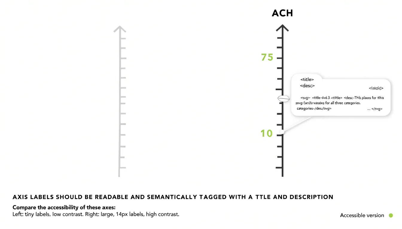
- High-contrast text: Axis labels, tick marks, and titles should have a contrast ratio of at least 4.5:1 against the background, as recommended by WCAG 2.1. Avoid low-contrast combinations like light gray on white, which can render axis information nearly invisible to users with low vision.
- Minimum legible font sizes: Use a minimum of 12 to 14 pixels for axis labels, depending on the context and display medium, so users on small screens or at a distance do not have to zoom or strain. Keep font sizing consistent across titles, labels, and tick marks.
- Screen-reader formatting: Provide semantic structure following modern standards such as WCAG 2.2. Use ARIA labels and roles to describe the chart’s type, axes, and data points. In SVG charts, include
<title>and<desc>elements, associate axis labels with their respective data through proper markup, and keep axis text selectable rather than embedded in images.
Frequently Asked Questions
Why should bar charts start at zero?
Bar charts encode value through bar length, so a zero baseline keeps each bar directly proportional to the quantity it represents. A zero baseline is required for any chart that encodes magnitude through length or area, including stacked and grouped bar charts, histograms, and area charts. Moving the baseline upward can make small differences look like large visual gaps.
Can I ever use a truncated axis?
Bar charts must anchor at zero, but line charts encode change in position and can use a non-zero baseline when starting at zero is impractical for large-magnitude time series. If using a non-zero range, clearly label the axis minimum, state the reason for the range, add a break symbol, and pair the trend line with a direct annotation of the actual values. Truncated axes can otherwise make small changes look dramatic and mislead readers.
What is a logarithmic scale useful for?
Logarithmic scales display data that spans several orders of magnitude and are especially valuable for exponential growth. They also allow comparing series with vastly different magnitudes on a single chart without one overwhelming the others. When preparing such a chart, label the axis with actual values at major tick marks and consider noting that the scale is logarithmic in the axis title.
Why are dual y-axis charts misleading?
Dual y-axes introduce perceptual traps because the crossing and divergence of lines can appear meaningful even though the intersection point is determined largely by arbitrary scale choices. Mismatched scales can also imply volatility where none exists, and readers rarely pause to check which line belongs to which axis. Small multiples or indexed values usually communicate the comparison with less risk of misreading.
How many gridlines should a chart have?
Aim for roughly four to seven gridlines across the full axis range, placed at intervals that match mental arithmetic such as 1, 2, 5, 10, 20, 25, or 50. Place axis labels at the same intervals so each reference line has an explicit value attached. If the gridlines are the first thing noticed, they are too prominent; if estimating a midpoint value requires squinting, they are too sparse.
Should I rotate axis labels?
Treat rotation as a last resort and redesign the chart so labels can stay horizontal. The simplest fix is often switching to a horizontal bar chart when category names are long, which places those names along the vertical axis where they read left to right naturally. Other options include truncating strategically, wrapping text, abbreviating, or reducing label density.
Tony Astor
Tony writes about data visualization and the tools people use to build charts and dashboards. More about Data Illustrator