Bubble Map: Showing Quantities by Location
 By Tony Astor ·

Bubble Map
A bubble map is a geographic visualization that places circles at specific locations and varies their size to represent quantity, making spatial clusters and volume concentration easy to see. Bubble size should scale by area, not radius, so viewers perceive magnitudes accurately, and color, tooltips, and transparency can encode secondary data and manage overlap.
Table of Contents
Bubble Map
A bubble map displays quantities at specific locations by varying the size of circles placed on a geographic map. This visual encoding allows viewers to quickly grasp spatial distribution patterns, such as geographic clusters and volume concentration, which are essential for understanding global supply chains. By examining the size and placement of bubbles, analysts can identify regions where activity is dense and where it is sparse.
For instance, a supply chain manager might use a bubble map to plot the volume of goods flowing through various ports. Large bubbles indicate major hubs with high throughput, while smaller bubbles represent minor ports. This immediate visual cue helps in recognizing concentration of volume and potential bottlenecks. The map also reveals clusters, where multiple large bubbles appear in close proximity, suggesting a regional dependence or a network of interconnected facilities. Such patterns are critical for risk assessment and strategic planning. For example, a cluster of large bubbles along a single coastline might indicate vulnerability to natural disasters or geopolitical tensions.
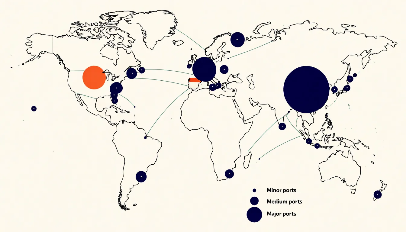
Bubble maps can also incorporate additional variables through color or labels, enabling a multidimensional view of supply chain data. However, their primary strength lies in conveying quantity and location simultaneously. In the context of global supply chains, bubble maps facilitate the identification of emerging markets, optimization of logistics routes, and monitoring of trade flows by highlighting where volume is concentrated and how spatial relationships influence the flow of goods.
Bubble Sizing
Mapping a numeric variable to the size of a circle is one of the most immediately legible ways to encode data in a bubble map, provided the translation from value to dimension is handled carefully. The core question is whether to drive the circle’s radius or its area.
Radius scaling is intuitive to compute: take the value, normalize it against the range in the dataset, and multiply by a maximum radius. The trouble is that a viewer perceives the circle’s area, not its radius, so doubling the value and doubling the radius produces a circle that looks roughly four times larger. This distortion makes differences between large values feel exaggerated and compresses the differences among small values.
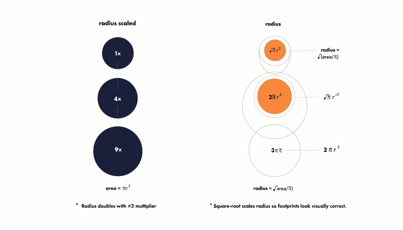
Area-based scaling corrects for this perceptual bias by solving for the radius that yields an area proportional to the value. In practice this means taking the square root of the normalized value before multiplying by the maximum radius. The result is a set of circles whose visible footprint matches the underlying numbers more faithfully, which matters when the chart is used to compare production yield across facilities or revenue across regions. A common convention is to define a maximum radius for the largest value and let all other circles fall out of the square-root formula, with a minimum radius floor so that small values remain clickable and visible.
The choice of scale also deserves attention. A linear mapping preserves absolute differences, while a square-root or logarithmic scale compresses wide ranges and keeps a handful of outliers from shrinking every other circle into an unreadable dot. Whichever route is chosen, adding a size legend with two or three reference circles gives readers a way to decode magnitudes directly. Annotating those examples with their actual values, rather than percentages, keeps the mapping honest and lets the bubble map function as a quantitative instrument rather than a decorative graphic.
Bubble Placement
Accurate bubble placement begins with reliable coordinate data, since every marker on a map is only as trustworthy as the latitude and longitude values behind it. Best practice starts with capturing positions in decimal degrees using the WGS84 datum, the standard understood by most mapping libraries and GPS devices. Mixing datums or recording coordinates in degrees, minutes, and seconds without conversion introduces small but persistent offsets that can push a bubble onto the wrong block or even the wrong city. Storing coordinates at six decimal places preserves precision to roughly ten centimeters, which is more than enough for most analytical maps while keeping file sizes manageable.
Once coordinates are in hand, the base map itself needs attention. Web maps commonly use the Web Mercator projection, and data plotted in a different projection will drift from the underlying streets and landmarks, especially at higher latitudes. Confirming that the coordinate reference system of the data matches that of the base map prevents this silent misalignment. It also helps to validate each point against known reference features, such as a coastline or a labeled intersection, before publishing the map.
Edge cases deserve special handling. Points that fall in the ocean because of a transposed latitude and longitude pair are a common error, and a quick check that latitudes sit between minus ninety and ninety and longitudes between minus one hundred eighty and one hundred eighty catches most of them. Antimeridian crossings and polar regions require additional care, since simple plotting routines can wrap lines and markers around the globe incorrectly. Finally, documenting the source, date, and datum of every coordinate set keeps the map reproducible and lets others audit the placement when questions arise.
Color Coding
By assigning colors to bubbles, you can represent a secondary metric alongside the primary data shown by bubble size and position. Hue and saturation are the two primary dimensions of color that can be manipulated to encode data:
- Hue—the distinct color itself, such as red, green, or blue—is ideal for categorical data. For instance, if your map displays oil production sites, you might use different hues to represent oil quality grades: light amber for high-quality crude, medium brown for standard grades, and dark brown for heavy sour crude. This immediately communicates the distribution of quality across regions without the need for additional labels or charts.
- Saturation—the intensity or purity of a color—is better suited for continuous or ordinal data. A highly saturated color draws the eye and suggests a high value, while a desaturated, muted tone indicates a lower value. For example, you could use saturation to represent ROI, with deep, vibrant green signaling high returns and pale green indicating lower returns. Similarly, risk factors could be shown with a gradient from pale yellow (low risk) to deep red (high risk).
The combination of hue and saturation allows for even more nuanced encoding. You might use hue to distinguish categories (e.g., different types of investments) and saturation to show the intensity of a metric within each category (e.g., risk level). This dual encoding enables viewers to compare both qualitative and quantitative aspects simultaneously.
Effective color coding requires careful consideration. Colors should be intuitive and culturally appropriate; for example, red often implies danger or high risk, while green suggests safety or positive outcomes. Additionally, ensure sufficient contrast between colors and use colorblind-friendly palettes with clear legends to maintain accessibility for colorblind viewers.
Overlap Management
Dense data sets create a predictable problem for bubble maps: when many observations share similar coordinates or fall within a small geographic radius, their circles begin to stack on top of one another and obscure the underlying pattern. Overlap management is the set of techniques that keeps these crowded regions readable while preserving the accuracy of what the map communicates.
- Transparency: By lowering the opacity of each bubble, overlapping marks blend into darker tones where density is highest, effectively turning the map into a visual histogram. A single pass of alpha blending can reveal hotspots that would otherwise look like one flat, opaque disc.
- Jittering: Adding a small, controlled random offset to each point spreads coincident bubbles into a tight constellation, allowing viewers to count individual observations rather than guess at a hidden stack. The technique works best when the displacement stays small enough that points remain anchored to their true location; larger offsets risk distorting geography for the sake of legibility.
- Clustering algorithms: Methods like grid-based aggregation or k-means group nearby points into a single representative bubble whose radius or color encodes the number of merged observations. This reduces the number of marks the eye must process while preserving the density signal. Interactive versions, where clusters split apart on zoom, balance overview and detail.
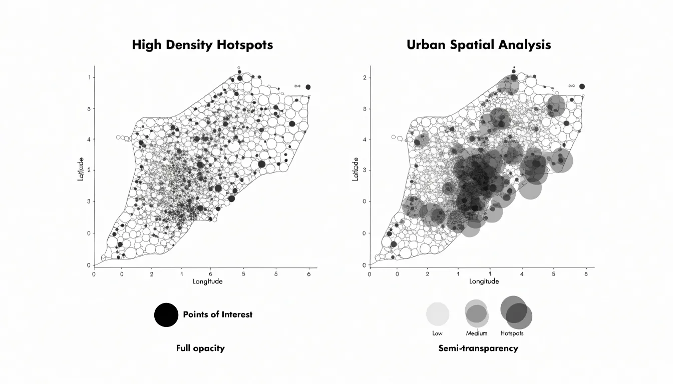
In practice, these techniques are often combined. Transparency handles mild overlap, jittering resolves tight coincidences, and clustering manages the extremes. The right choice depends on the data’s scale, the map’s purpose, and the audience’s need for individual versus aggregate readings.
Data Preparation
Cleaning geographic numbers before mapping begins with a reliable geocoding step. Take each address or location string in the dataset and pass it through a geocoding service or your internal reference table, converting text into latitude and longitude pairs. Where possible, append a postal code or region to the query so ambiguous names resolve correctly. Record the precision level returned by the geocoder, such as rooftop, street, or locality, and flag low-precision results for manual review.
Once coordinates exist, standardize location names across the dataset. Trim whitespace, unify capitalization, expand abbreviations, and settle on one spelling for each place. Apply the same normalization to country and region fields so that entries like USA, U.S.A., and United States collapse into a single value. A lookup table of canonical names makes this consistent and repeatable.
Next, remove null and invalid values. Rows with missing coordinates cannot be placed on a map, and coordinates outside valid ranges indicate data entry problems. Filter out these records and log how many were dropped and why, keeping an audit trail for later review. Check for duplicate entries that would overstate a location’s weight in the map. Run a consistency pass comparing the coordinate against the stated region to catch mismatches.
Finally, validate the cleaned dataset by counting rows, verifying coordinate ranges, and spot-checking a sample of locations against their source values. Store the cleaned output separately from the raw data so the process can be rerun, and document each transformation step for future updates.
Area Scaling
Perceptual research consistently shows that people judge the size of filled shapes by area rather than by linear extent, which makes area the honest channel for quantitative comparison. As established in the Bubble Sizing section, scaling radius linearly with a data value causes the area to grow with the square of the value, inflating the largest bubbles far beyond their true proportion and shrinking the smallest until they are nearly invisible.
Practically, implementing area scaling means computing the radius as a constant multiplied by the square root of the data value, then tuning that constant so the largest bubble fits the available space without overwhelming its neighbors. Because surface area grows with the square of the radius, this square-root transformation ensures that a bubble covering twice the area stands for twice the metric. The resulting map lets viewers read relative magnitudes at a glance, trusting that the visual difference they perceive matches the numerical difference in the data rather than an artifact of linear scaling.
Interactive Maps
Interactive maps turn a static visualization into a working instrument for exploration. The core mechanism is the hover interaction: when a user moves their cursor over a bubble, region, or marker, a tooltip appears with the exact figures behind that shape. A bubble whose size encodes hundreds of suppliers becomes legible only when the precise count surfaces on hover, and that number arrives alongside the supplier names and metadata that give the aggregate real meaning. Each tooltip can show the total count, a short list of the suppliers represented, and descriptive fields such as category, region, or reporting period. This lets users verify what they are seeing instead of estimating from circle area, a task humans perform poorly even with well-designed legends.
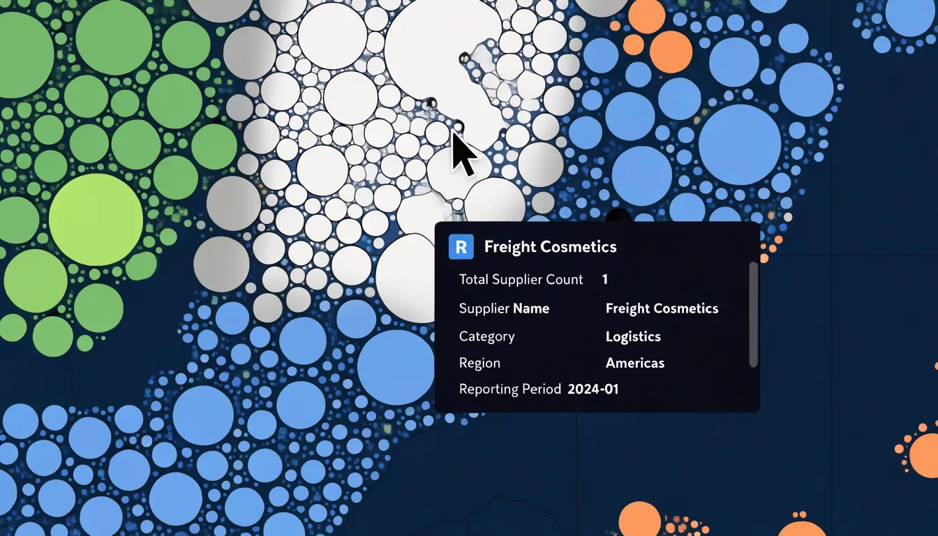
Implementation begins with binding data to each map element so the tooltip has a reliable source. A common approach is to attach a data object to every rendered shape and populate the tooltip from that object on pointer events. Tooltips should follow the cursor, stay within the viewport, and remain readable when several bubbles cluster closely together. For touch devices, where hover does not exist, a tap can open a popup with identical content, and a close control keeps the interaction manageable. Keyboard focus should also trigger the same disclosure so the information is not locked behind a pointer.
Performance matters once a map carries thousands of elements. Listening on a single container and determining the target from the event keeps handlers lean, and rendering tooltips as reusable DOM nodes avoids rebuilding markup on every hover. Because tooltips expose individual records, they also raise privacy questions: supplier names should appear only where publication is appropriate, with aggregation or anonymization applied elsewhere. Handled with care, hover disclosure makes the map trustworthy, since every visual impression can be checked against the underlying data.
Time Lapses
Animating spatial-temporal data transforms a static bubble map into a narrative that unfolds over time. A time lapse works by stepping through successive years, redrawing the map at each interval so that bubble positions, sizes, and colors shift in sequence. When the animation is calibrated to a steady frame rate, viewers can follow individual regions or suppliers across the full arc of the dataset, watching how their prominence rises, stabilizes, or fades. This is especially useful for illustrating shift patterns in sourcing, where production hubs may migrate from one part of the world to another as labor costs, trade agreements, or logistics constraints change. A single moment on the timeline captures a snapshot; the sequence reveals the trajectory.
Sales growth benefits from the same treatment. A company operating across many markets can chart revenue by location and let the animation reveal which territories accelerate, which plateau, and where demand is quietly emerging. Because the human eye is drawn to motion, gradual color transitions and growing bubbles communicate momentum without requiring the viewer to compare a stack of static maps side by side. Climate impacts follow a similar logic: temperature anomalies, emissions, or extreme-weather indicators can be plotted at each year and animated to show how effects concentrate and spread across geographies.
The design of a time lapse matters as much as the data. Consistent scaling across all frames prevents misleading jumps, clear year labels anchor the viewer in time, and controls for pausing or scrubbing let audiences linger on moments of interest. The result is a compact visual story that compresses decades of change into a short, legible sequence.
Regional Analysis
Spatial coverage maps turn sourcing strategy into something visible and testable. By plotting each known supplier, farm, wild-harvest site, and processing facility onto a geographic base layer, teams can see at a glance where botanical supply chains cluster and where they thin out. Overlaying demand signals, such as regional sales volume or forecast growth, sharpens the picture further: a dense cluster of suppliers near a low-demand area reveals surplus, while a high-demand region ringed by distant or few sources exposes a genuine gap. The map becomes a diagnostic instrument, converting a spreadsheet of vendor addresses into a structured view of coverage, distance, and concentration.
The next step is layering in context that explains why a gap exists. Protected land boundaries, climate zones, elevation bands, transport corridors, and port access all shape whether an underserved market is a real opportunity or simply unsuitable terrain for a given botanical. A region may show no suppliers because the species cannot grow there, or because roads and cold-chain infrastructure are absent, or because no one has yet built relationships with local growers. Distinguishing these cases is where the map earns its value. Pairing coverage layers with harvest calendars and species suitability data helps identify where a missing supply chain could realistically be developed rather than merely observed.
Coverage maps also support portfolio-level decisions. Comparing maps across several botanicals reveals shared gaps, letting a single investment in regional sourcing infrastructure serve multiple product lines. Tracking the maps over successive seasons shows whether coverage is widening, consolidating, or drifting, which informs risk planning around concentration and single-origin dependence. Gaps flagged this way become concrete research tasks: scouting visits, agronomic assessments, or conversations with regional cooperatives. Used consistently, spatial coverage mapping moves sourcing from reactive vendor management toward a deliberate, geography-aware plan for where supply needs to exist next.
Mobile Adjustments
Small screens impose hard physical limits on what a map can show before it becomes cluttered or unusable. Touch targets sit at the center of this problem. A data point, marker, or interactive region that reads comfortably on a desktop monitor shrinks to a few pixels on a phone, and fingers are far less precise than a cursor. Designers address this by enlarging tappable areas beyond the visible symbol, spacing interactive elements so adjacent targets do not overlap, and reserving the smallest touch zones for secondary actions. The finger becomes the unit of measurement, and every control is sized and positioned with that in mind.
Zoom behavior needs equal attention. Responsive zooming means the map adapts its scale and detail to the device rather than simply shrinking a desktop view. Pinch gestures should feel immediate, with smooth transitions between zoom levels and sensible limits that keep users from drifting into empty space or overwhelming detail. Automatic framing helps here, centering the relevant data at a scale appropriate to the viewport so that the first thing a user sees is legible and complete.
Basemap simplification rounds out the adjustments. Detailed labels, fine-grained roads, and dense texture that work well at large sizes can turn into visual noise on a handset. A simplified basemap strips away competing elements, keeps only the labels and features necessary for orientation, and lets the data layer stand out. Combined, these choices produce a mobile map that feels native to the device, where targets are easy to hit, zooming feels natural, and the underlying geography supports the story instead of crowding it.
Design Practices
When designing bubble maps, color and typography are the primary tools for conveying information clearly. Start with an accessible color palette that meets WCAG contrast guidelines. Use a limited set of colors—perhaps three to five—to represent categories or values, and ensure each color has sufficient contrast against the background. Avoid relying solely on hue to differentiate bubbles; incorporate patterns or labels for users with color vision deficiencies. For sequential data, choose a single-hue gradient that progresses from light to dark, with clear differentiation between steps. Test your palette with online contrast checkers to guarantee readability.
Typography should establish a clear visual hierarchy. Use a limited number of font sizes and weights: for example, a larger, bold font for bubble labels and a smaller, regular font for secondary information. Ensure text is legible at small sizes by choosing a clean sans-serif typeface and maintaining a contrast ratio of at least 4.5:1 between text and background. Avoid placing text directly over busy areas of the map; instead, use labels with sufficient padding or place text in a consistent location relative to the bubble. For bubble labels, consider adding a subtle text shadow or halo to improve legibility over varied backgrounds. Keep text concise to guide the viewer’s eye to the most important data points.
Common Mistakes
When creating bubble maps, common mistakes often stem from how sizes, labels, and legends are handled:
- Exaggerated radius scaling: Setting the radius proportional to the data value rather than scaling by area (or using a square root transformation for the radius) causes viewers to overestimate the importance of large values.
- Overlapping text labels: When bubbles are close together, labels can collide, become unreadable, or obscure the data they are meant to clarify. Techniques such as leader lines, label repositioning, or interactive tooltips can help, along with prioritizing labels for key bubbles.
- Ambiguous legend keys: A legend that shows bubbles of different sizes without indicating the exact values they represent leaves viewers guessing. Always include specific reference values (e.g., circles for 10, 100, 1000) and ensure the legend is clearly tied to the visual encoding.
- Redundant encoding: Avoid using color and size to represent the same variable, as this can create confusion.
Real World Examples
Several leading essential oil brands have adopted interactive bubble maps as a core tool for documenting and communicating their sourcing and distribution practices:
- Lavender in Provence: One producer represents each supplier farm as a bubble sized according to annual yield and colored by certification status. Clicking a bubble reveals harvest dates, distillation records, and fair-wage agreements, giving retailers and consumers a transparent view of the supply chain from field to bottle.
- Frankincense and myrrh in Oman, Somalia, and Yemen: A cooperative maps each harvesting community as a bubble, with size reflecting the volume purchased and hue indicating the cooperative’s sustainability rating. Because the map updates as new harvests are recorded, partners can see seasonal shifts in real time and adjust purchasing decisions accordingly.
- Distribution in Europe and North America: A mid-sized essential oil company uses a bubble map to visualize shipment volumes by region, with bubble size tracking units moved and clustering revealing where demand concentrates. This enables the logistics team to identify bottlenecks at specific ports and reallocate inventory before shortages occur.
- Tea tree oil in Australia: A brand layers sourcing bubbles over distribution bubbles to show how raw material flows from growers to processing facilities and onward to retail partners.
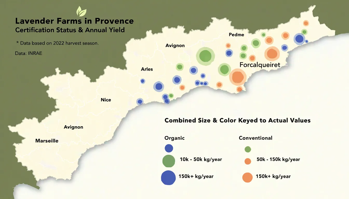
Together, these case studies demonstrate how a single visual format accommodates sourcing transparency, sustainability auditing, and logistics oversight. The common thread is that each brand treats the map as a living document rather than a static graphic, updating data frequently and sharing access with stakeholders who need it. This practice builds trust with conscious consumers and gives operations teams a shared reference point for decisions.
Final Review
Before a bubble map leaves your hands, a final review pass protects both your credibility and your audience’s ability to read the data correctly.
- Verify geocoordinates: Open the project file and confirm that every plotted point sits where it should on the basemap. Coordinates transposed from latitude to longitude, or copied with a stray decimal, will place a city in the wrong hemisphere, and the error can hide behind an otherwise convincing cluster. Zoom in on a handful of known locations and check the bubble centers against recognizable landmarks or administrative boundaries.
- Audit the legend: Each size class or color band should map to a specific numeric range stated plainly in the legend text. Verify that the smallest and largest bubbles on the map correspond to the values the legend promises, and that no bubble falls outside the defined classes. A legend that understates its top category misleads readers about magnitude even when the underlying numbers are sound.
- Check scale ratios: Confirm that the visual size of each bubble scales proportionally to the value it represents, whether by area or by radius, and that this choice is documented in the caption. Check the map’s geographic scale bar as well, since projection distortion can make distant bubbles appear deceptively large or small.
- Review data integrity: Reconcile the totals in the map against the source dataset, spot-check individual records, and confirm that null or zero values are rendered distinctly rather than dropped silently. Note the data’s collection date and any filtering applied.
A short checklist completed consistently before each release catches the errors that are hardest to see once the map is finished.
Dashboard Overview
A spatial bubble map becomes far more useful when it sits inside a dashboard alongside other views. Bar charts, summary KPIs, and filter controls each answer a different kind of question, and placing them next to the map lets readers move between geographic patterns and quantitative comparisons without losing context.
A bubble map shows where values cluster and how magnitudes vary across locations, while a bar chart ranks the same categories or regions in a straightforward order. Seeing both at once means a viewer can spot an outlier on the map and immediately check its rank in the chart, confirming whether a large bubble represents a genuine leader or simply a dense area with many small contributors.
Summary KPIs anchor the whole view by surfacing totals such as overall volume, average value per location, or the count of active regions. These headline numbers give readers an immediate sense of scale before they dive into detail, and they update as filters change, so the dashboard tells a coherent story rather than presenting disconnected panels. Filter controls—such as a date range selector, a category toggle, or a region dropdown—tie the components together, letting users narrow the data and watch every view respond in step.
Layout matters as well. Placing the map in a prominent position, with KPIs across the top and charts to the side, creates a natural reading path from overview to detail. Consistent colors, bubble sizing, tooltips, and shared legends across all panels help viewers track the same category from map to chart without reinterpreting the visual language. When these elements work together, the KPIs frame the scale, the map reveals geography, the charts provide comparison, and the filters let each reader pursue their own line of inquiry.
Frequently Asked Questions
What is a bubble map used for?
A bubble map displays quantities at specific locations by varying circle sizes on a geographic map, making clusters, volume concentration, and spatial distribution easy to see. In supply chains, it can show port throughput, identify major hubs and bottlenecks, and support risk assessment and strategic planning.
Should bubble size be scaled by radius or area?
Use area-based scaling, because viewers perceive a circle’s area rather than its radius; scaling radius linearly exaggerates large values. Area scaling uses the square root of the normalized value before multiplying by the maximum radius.
What coordinate system and datum should I use for bubble placement?
Best practice is to capture positions in decimal degrees using the WGS84 datum and confirm that the data’s coordinate reference system matches the base map. Validate each point against known reference features and check that latitudes and longitudes fall within valid ranges.
How can I manage overlapping bubbles on a dense map?
Use transparency to reveal density, jittering to spread coincident bubbles slightly, or clustering algorithms to group nearby points into representative bubbles. These techniques are often combined, with clustering managing the extremes.
How should I use hue and saturation when color coding bubbles?
Hue is ideal for categorical data, while saturation is better for continuous or ordinal data; combining them can encode both category and intensity. Ensure sufficient contrast and use colorblind-friendly palettes with clear legends for accessibility.
How should a bubble map be adjusted for mobile screens?
Enlarge tappable areas beyond the visible symbol, space interactive elements so adjacent targets do not overlap, and use responsive zoom with smooth pinch gestures and sensible limits. Simplify the basemap so detailed labels and roads do not become visual noise.
Tony Astor
Tony writes about data visualization and the tools people use to build charts and dashboards. More about Data Illustrator