Bubble Chart: Adding a Third Variable to a Scatter Plot
 By Tony Astor ·

Bubble Chart
A bubble chart is a scatter plot that encodes a third numeric variable as the size of each circle, keeping x and y positions for the first two variables. Bubble areas must be scaled proportionally to values using radius = √(k × value), since mapping values to radius inflates larger bubbles and distorts comparisons.
Table of Contents
- Scatter Plot Basics
- Bubble Charts
- Sizing Bubbles
- When to Use Bubble Charts
- Setting Up Axes
- Adding Color Encoding
- Preparing Your Data
- Designing for Readability
- Transparency and Layering
- Interactive Features
- Real World Examples
- Avoiding Misleading Visuals
- Mobile Layouts
- Presenting Multi-Variable Data
- Final Checklist
Scatter Plot Basics
A scatter plot places each observation as a single point on a two-dimensional plane defined by a horizontal X axis and a vertical Y axis. Each point represents one record, with its horizontal position determined by the value of the first variable and its vertical position determined by the value of the second. This simple mapping turns a table of paired numbers into a visual field where patterns become immediately apparent. When the points drift upward from left to right, the two variables tend to rise together; when they drift downward, one tends to fall as the other rises; when they form a shapeless cloud, the variables appear largely independent.
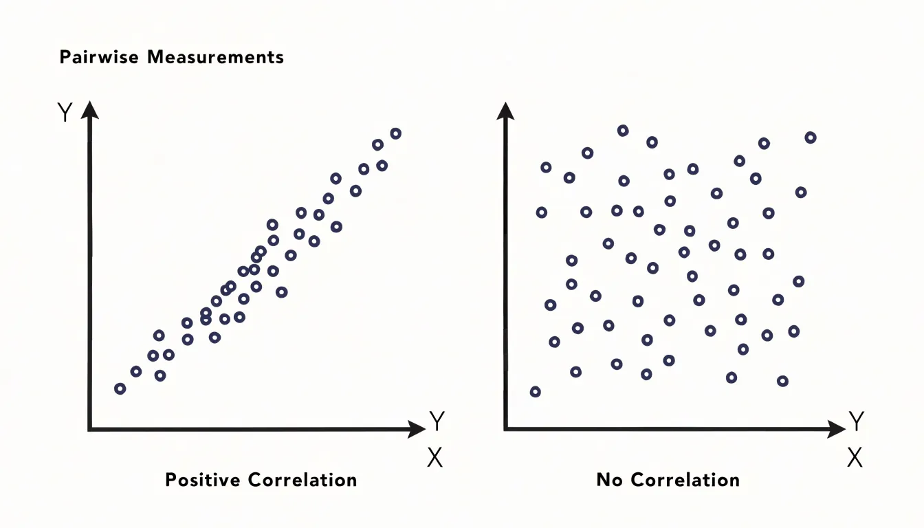
The power of the scatter plot lies in how much structure the human eye can read from that point cloud. Analysts look for the overall trend, the direction and tightness of the relationship, and the presence of clusters where points gather in distinct groups. Equally important is spotting outliers, individual points that sit far from the main body of data and often signal measurement errors, unusual cases, or interesting anomalies worth investigating. The shape of the cloud also matters: a curved arrangement suggests a nonlinear relationship that a simple correlation coefficient might miss, while a fan shape reveals that variability changes across the range of the X variable.
Correlation coefficients quantify the strength and direction of the linear association, but the plot reveals the context the number cannot capture. A single statistic can describe a relationship that is actually driven by a few extreme points, or that splits into two separate subgroups. Seeing the points makes these situations visible. These mechanics form the starting point for more elaborate visualizations, where color, size, or motion can encode additional variables on top of the same X-Y foundation.
Bubble Charts
A bubble chart extends the scatter plot by encoding a third numeric variable in the size of each plotted circle. Where a standard scatter plot places points according to two axes, the bubble chart keeps those same x and y positions while allowing the circle to grow or shrink in proportion to a separate value, carrying three dimensions of information within a single flat view. Readers can scan the chart and distinguish small, medium, and large circles at a glance, associating that visual difference with a corresponding magnitude in the underlying data.
Size is one of the most immediate visual cues available, and the human eye is quick to compare circles of different diameters without needing a legend at every glance. A circle visibly larger than its neighbors signals a bigger value, whether that value represents revenue, population, transaction count, or any other quantity worth tracking. This intuitive mapping lets the chart communicate numeric magnitude in a way that feels direct and accessible, even to viewers encountering the data for the first time.
Designers pair the size channel with position, color, and labeling to keep the chart readable as circles grow larger. Overlapping bubbles can obscure one another, so careful choices about scale ranges, opacity, and layering help preserve clarity. Legends that map circle sizes to representative values give viewers a reference point for interpretation.
Sizing Bubbles
Sizing bubbles accurately requires a deliberate choice about which geometric property of the circle carries the data. The natural instinct is to map a value onto the radius, since radius is the most visible dimension of a circle and doubling it feels like doubling the quantity. That instinct produces a systematic and surprisingly large error. A circle’s area grows with the square of its radius, so doubling the radius quadruples the area. If a bubble representing 20 is drawn with twice the radius of one representing 10, the larger bubble covers four times the ink and reads, at a glance, as roughly four times the value. The viewer perceives area, not radius, so mapping values onto radius silently inflates every value above the baseline and compresses the gap between large and small observations.
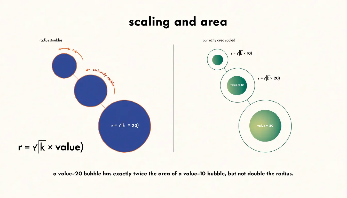
The correct approach maps the value onto the area itself. Starting from the area formula A = πr², solving for the radius gives r = √(A/π). In practice, a chart designer picks a scale factor k that converts data units into area units, then computes each bubble’s radius as r = √(k × value). The square root is the essential step: it counteracts the quadratic relationship between radius and area so that a value twice as large yields a bubble with exactly twice the area and therefore twice the visual weight.
This mathematical adjustment keeps proportions honest: twofold differences in the data look like twofold differences on the page, and a tenfold difference looks tenfold, regardless of the absolute magnitudes involved. Range also warrants attention, since very large values can dominate the canvas and crowd out smaller bubbles; a square-root or logarithmic transformation of the values may be preferable when the data spans several orders of magnitude. Whatever transformation is chosen, the scaling rule should be applied consistently across every bubble and documented in the chart’s caption or legend so that readers can interpret relative sizes with confidence.
When to Use Bubble Charts
Bubble charts are most effective when you have three continuous variables for each data point and want to explore how they interact. This makes them ideal for datasets where the magnitude of a third factor adds meaningful context—for example, comparing countries by GDP per capita (x-axis), life expectancy (y-axis), and population (bubble size), or products by price, customer satisfaction, and sales volume. In such cases, the relative sizes of bubbles quickly convey which items are dominant in the third dimension, revealing patterns that would be lost in a standard scatter plot.
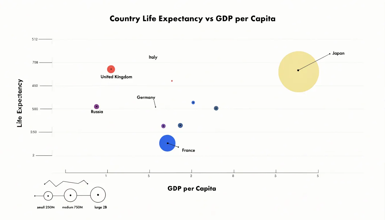
Optimal datasets typically have a moderate number of points—enough to show trends, clusters, or outliers across all three dimensions simultaneously, but not so many that bubbles overlap excessively. They also benefit from a size range that is not so extreme that small bubbles become invisible or large ones overwhelm the chart.
Conversely, bubble charts are a poor fit in several situations:
- Sparse datasets: With only a handful of points, the visual impact of size differences is diminished and trends are hard to discern.
- Overcrowded or uniform datasets: Too many points or bubbles of very similar sizes create clutter and make area comparisons difficult, especially since human perception of area is less precise than that of length.
- Categorical third variables: When the third variable is categorical or has limited variation, a bubble chart adds little value over a color-coded scatter plot.
Setting Up Axes
Setting up the axes is where a bubble chart either earns the reader’s trust or quietly loses it. Begin with the horizontal and vertical axes, since these carry the first two variables and anchor every other dimension of the chart. Choose the scale family before drawing anything. When a variable is distributed roughly evenly across its range, a linear scale keeps distances intuitive and comparisons honest. When values cluster at the low end and stretch into a long tail, a logarithmic scale compresses that tail and reveals structure that a linear axis would flatten into an unreadable smear at one edge. Inspect the distribution of each variable—histograms or summary statistics will do—and let the shape of the data decide.
Labeling deserves equal care. Place a short, descriptive label on each axis that names the variable and includes its units, such as “GDP per capita (USD)” rather than a bare “GDP.” Tick marks should be spaced at regular, round intervals so readers can estimate values without arithmetic, and gridlines should be subtle enough to guide the eye without competing with the bubbles themselves. Where a transformed scale is in use, make that explicit in the label or with a clear notation so no reader misreads a logged gap as a linear one.
Zero-baselining is the third pillar. Where position encodes value, starting the axis at zero prevents small differences from being visually exaggerated and keeps the relationship between the two plotted variables in proportion. When a zero origin is impractical, say so and mark the axis break or truncated range clearly. Consistency across both axes, thoughtful tick density, and honest origins together ensure the chart communicates the data’s true shape at a glance.
Adding Color Encoding
Adding color to a bubble chart introduces a fourth dimension of information alongside x-position, y-position, and bubble size. A distinct color palette can map a categorical variable, with each hue assigned to one category. When the added variable is continuous, a sequential or diverging gradient works better, letting the eye read subtle shifts in value across the chart without needing extra labels or crowding the plot area. The choice between discrete hues and a smooth gradient depends on the nature of the underlying data and the number of distinct values the reader needs to distinguish.
Selecting an accessible palette matters as much as the encoding itself. Contrast between adjacent hues should be strong enough that readers can tell categories apart at a glance, even when bubbles sit close together or overlap. Palettes based on lightness variation as well as hue variation tend to hold up better for readers with color vision deficiencies, since they remain distinguishable when the red-green channel is unreliable. Avoiding red and green pairings as the sole differentiator, and steering clear of low-saturation pastels that fade against a white background, keeps the chart readable for a wider audience.
The number of colors should stay modest. Beyond six or seven distinct hues, recognition slows and legend matching becomes a chore. Where more categories exist, grouping smaller ones into an ‘other’ shade preserves clarity. Testing the chosen scheme under simulated color blindness and on both light and dark backgrounds catches problems before publication. Consistent application of the palette across the chart, with a clear legend or direct labels, ensures that color supports the reading of the data rather than competing with it.
Preparing Your Data
Preparing your data before building a bubble chart determines how faithfully the final visualization represents reality. The first task is to inspect every numeric column for missing values, since empty cells can distort axis scaling or cause charting tools to silently drop records. Decide on a consistent strategy: remove rows with missing critical values, substitute a documented default, or flag the gaps so viewers understand where the data is incomplete. Consistency matters more than the specific choice.
Next, examine extreme outliers. A single order-of-magnitude outlier can compress the rest of the points into an unreadable cluster, so review each unusually large or small value and decide whether it reflects a genuine observation or a data entry error. Where outliers are valid, consider applying a log transformation or capping values at a documented threshold so the chart’s axis range communicates meaningful variation. Record exactly what was adjusted, because viewers will read bubble size and position as literal measures.
Numeric formatting is equally important. Strip currency symbols, thousands separators, percent signs, and text annotations from columns so the charting tool can interpret them as numbers rather than strings. Where units differ, convert everything to a single unit before import, and keep decimal precision consistent so aggregated values behave predictably. Ensure that each column has a clear header, that rows represent individual observations, and that there are no merged cells or summary rows embedded in the data region. These structural details prevent the tool from misreading the table on import.
Designing for Readability
When many data points occupy similar values, bubbles tend to collide and merge into an unreadable mass. A first practical technique is jittering: applying a small, controlled random offset to each bubble’s position along both axes. The offset should stay well below the scale of meaningful differences in the data, so the underlying pattern remains legible while individual circles regain distinct outlines. Consistent jitter, applied once and stored, keeps the chart stable across renders rather than shimmering each time it loads.
Selective labeling complements this by refusing to annotate every bubble. Instead, labels attach only to the largest values, to outliers, or to points above a size threshold, with the remainder identified through hover states or a linked legend. Alternating label placement above and below bubbles, or drawing short leader lines to a margin, further reduces collisions between text and circles. A useful rule is to cap visible labels at a fixed count and rank candidates by importance.
Adjusting chart bounds is another lever. Expanding the domain slightly beyond the data range gives crowded edge bubbles breathing room, while adding padding around the plot area prevents clipping. In dense regions, temporarily increasing the bubble size range spreads radius values apart, making small differences visible without enlarging every mark. Combining a modest opacity setting with a thin stroke helps overlapping bubbles read as layered shapes rather than a single blob.
Finally, consider aggregation when crowding is severe: group nearby points into a single larger bubble, or provide a zoom interaction that expands a dense cluster.
Transparency and Layering
In dense bubble charts, the largest bubbles can easily sit on top and obscure everything beneath them. Alpha transparency is the primary tool for solving this problem. By setting the fill of each bubble to a partially transparent value, typically somewhere between 0.3 and 0.7 depending on how many overlapping points exist, every mark contributes color to the region it covers while still allowing the marks underneath to show through. Where bubbles overlap, the colors blend, and the resulting darker patches become an intuitive visual signal of high density. A viewer can see at a glance where many observations coincide, even when individual bubbles are only a few pixels across.

Transparency works best when paired with deliberate layer ordering. Browsers and charting libraries draw elements in the order they appear in the document, so the last bubble rendered sits on top. If large bubbles are drawn after small ones, the small bubbles vanish beneath them. Sorting by radius so that the largest bubbles render first and the smallest render last keeps every point visible, regardless of how tightly the cluster packs together. The z-index of each mark can be assigned from the same sort, giving explicit control over the stacking order rather than relying on the incidental order of the data array.
A clinician reviewing a dense scatter of patient outcomes and a product analyst examining transaction volumes both benefit from the same principle: no data point should disappear simply because it happens to sit near larger neighbors. Opacity ensures that overlap reads as accumulated presence rather than occlusion, and layer sorting guarantees that the smallest marks—often the most specific and interesting observations—remain perceptible in the final image.
Interactive Features
Interactive features turn static bubble charts into exploratory tools that balance a clean overview with on-demand detail:
- Hover tooltips: When a viewer hovers over a bubble, a custom tooltip can reveal exact x and y values, the bubble’s size metric, category, and additional data fields. Immediate access to precise numbers eliminates error-prone estimation from axes or circle areas while keeping permanent labels off the canvas.
- Dynamic filtering: Interactive controls let viewers select specific categories or value ranges, updating the chart in real time to show only relevant bubbles for focused analysis.
- Interactive legends: Clicking legend items to toggle categories on and off highlights patterns or isolates comparisons without cluttering the visual space.
Real World Examples
Bubble charts excel at comparing products across three variables simultaneously, revealing strategic trade-offs and market opportunities:
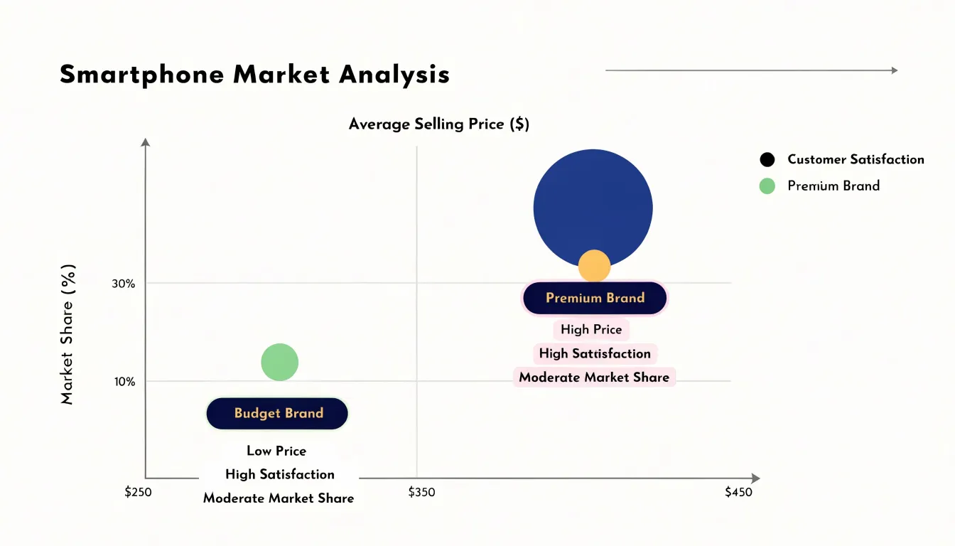
- Smartphones: Plotting average selling price on the x-axis, market share on the y-axis, and customer satisfaction as bubble size shows which brands dominate. A premium brand like Apple might appear as a large bubble (high satisfaction) positioned high on price but moderate on share, while a budget brand like Xiaomi could show a smaller bubble (lower satisfaction) with low price and high share. A brand with high satisfaction but low share may need to adjust pricing or marketing to expand, while a high-share brand with low satisfaction risks erosion.
- Laptops: Using the same three variables reveals market clusters. A cluster of mid-priced laptops with high satisfaction and moderate share indicates a sweet spot for value, whereas a high-priced laptop with high satisfaction and tiny share suggests a niche premium product. Businesses can also spot white space, such as an underserved high-satisfaction, low-price segment.
- Electric vehicles: Comparing newer entrants against established players by price, market share, and satisfaction highlights competitive threats—for instance, a large bubble (high satisfaction) at a lower price and growing share signals a disruptive entrant.
Avoiding Misleading Visuals
Beyond the radius-versus-area sizing trap covered earlier, several baseline and scaling pitfalls can distort how readers compare bubbles. Authors should state the size mapping explicitly in a caption or legend and supply a size key with reference bubbles so readers can calibrate their perception against known values.
Zero-point clipping presents a related problem. Truncating the size scale, or starting bubble sizes from an arbitrary minimum rather than from zero, compresses the low end and inflates small differences into dramatic contrasts. A value of two and a value of three can appear wildly apart when both are rendered against a shifted baseline. Honest representation begins sizes at zero—or clearly flags any departure from that baseline—and keeps a fixed scale across all panels of a multi-chart figure so that readers can compare regions without hidden rescaling.
Finally, while sorting smaller bubbles to the top and adding transparency prevents occlusion, transparent fills introduce a secondary complication: darker overlap regions can be mistaken for higher values or a distinct category. Documenting the fill opacity alongside the size mapping helps readers interpret overlapping clusters accurately.
Mobile Layouts
A desktop bubble chart’s strength—packing position, size, and color into one view—makes it difficult to read on a phone. The available canvas shrinks to a narrow portrait rectangle, labels compete for the same few square inches, and a finger replaces the precise cursor as the pointing device. Responsive design for mobile bubble charts begins with accepting these spatial constraints and reworking the interactions around them rather than merely scaling the desktop version down.
Touch-friendly tooltips are the first practical adaptation. On a phone there is no hover state, so tooltips must be triggered by a tap and designed to appear without covering the bubble being inspected. Anchoring the tooltip near the tapped point while nudging it away from screen edges keeps the information visible, and a generous tap target around each bubble reduces mis-taps in dense clusters.
Simplified legend placements follow the same logic. A legend that occupies a column beside the chart works on wide screens but steals scarce width on a phone, so moving it into a horizontal strip above or below the plotting area, or collapsing it into a toggleable sheet, frees vertical space for the bubbles themselves. Filtering by series through the legend can also double as a way to reduce clutter on demand.
Legibility ties these choices together. Bubble sizes need minimum radii so small values remain tappable, static labels should be limited to key points, and axis ticks can be thinned to avoid crowding.
Presenting Multi-Variable Data
When presenting a multi-variable bubble chart to an audience, the goal shifts from showing data to guiding attention through a dense field of circles. Two techniques help turn that complexity into a clear sequence:
- Callout annotations: A short text label placed beside a specific bubble acts as the narrator’s voice, explaining why a standout performer, outlier, or unusual cluster matters. Well-placed callouts sit close to the bubble they describe, use restrained typography, and answer the question a viewer would naturally ask at that moment.
- Focused highlight states: Dimming most bubbles while bringing one group or category to full opacity creates a visual spotlight. A sequence of highlight states across slides or animation frames can build a narrative step by step: first showing the full field, then emphasizing top performers, and finally singling out a specific segment for comparison. Simple color saturation and opacity changes work best; heavy outlines or flashing effects tend to distract from the underlying pattern.
Final Checklist
Before publishing or sharing a bubble chart, run through a final quality control review:
- Scale accuracy: Confirm that axis ranges and size encodings reflect underlying values proportionally, zero baselines are handled deliberately, and radii are scaled by area rather than diameter. Cross-check a handful of plotted points against the source data.
- Color contrast: Verify that overlapping bubbles remain distinguishable, the palette works on both light and dark backgrounds, and adjacent categories have sufficient luminance contrast for readers with color vision deficiencies.
- Accessibility: Provide a concise text summary or data table alongside the chart, confirm that interactive elements have keyboard support and descriptive labels, and ensure no meaning is conveyed by color alone so screen reader users can reach the same insights.
- Label legibility: Check that axis titles, tick values, and annotations are readable at final display size, labels do not collide, and the legend explains every encoding. Trim redundant text.
- Cross-format testing: Inspect the chart on a small mobile screen as well as in print or exported image formats to catch layout shifts.
Frequently Asked Questions
How should I size bubbles in a bubble chart?
Map each value to the bubble’s area rather than its radius. The article explains that radius is calculated as r = √(k × value) because area grows with the square of the radius, so radius-based sizing inflates visual differences.
When should I use a bubble chart?
Use a bubble chart when you have three continuous variables for each point and want to explore how they interact, especially with a moderate number of points. Avoid it for sparse datasets, overcrowded or uniform data, or when the third variable is categorical.
Should bubble chart axes start at zero?
Where position encodes value, starting the axis at zero prevents small differences from being visually exaggerated. If a zero origin is impractical, mark the axis break or truncated range clearly.
What does color add to a bubble chart, and how should I choose a palette?
Color adds a fourth dimension: use distinct hues for categorical variables and a sequential or diverging gradient for continuous ones. Keep the number of colors modest, use accessible contrast, and avoid red-green pairings as the sole differentiator.
How can I keep overlapping bubbles from hiding each other?
Use alpha transparency, typically around 0.3 to 0.7 depending on overlap, and draw the largest bubbles first so smaller ones remain visible on top. Document the opacity because darker overlap regions can be mistaken for higher values or a distinct category.
How do I make a bubble chart readable on mobile?
Trigger tooltips by tap rather than hover, move or collapse the legend to free space, set minimum bubble radii for tappability, limit static labels, and thin axis ticks.
Tony Astor
Tony writes about data visualization and the tools people use to build charts and dashboards. More about Data Illustrator