Box Plot vs Violin Plot: What Each Reveals
 By Tony Astor ·
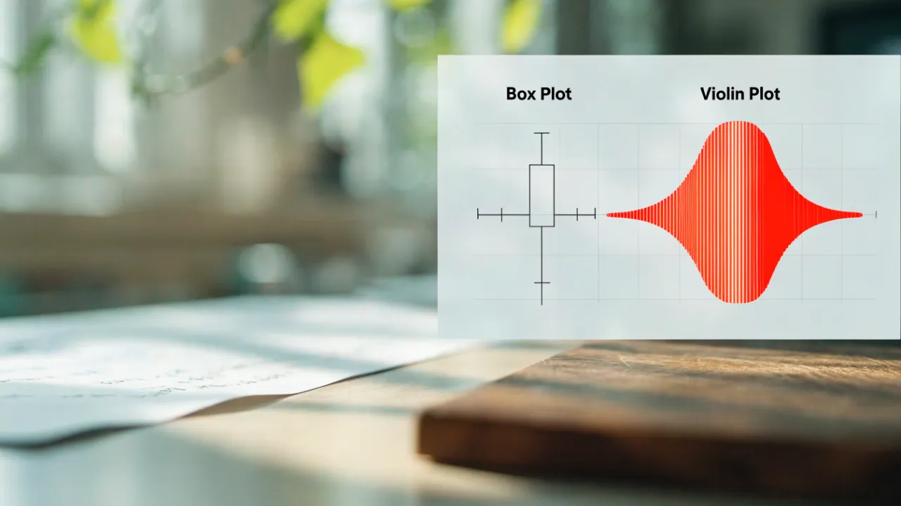
Box Plot vs Violin Plot
A box plot summarizes a distribution using five statistics (minimum, Q1, median, Q3, maximum) and excels at compact group comparisons, but it hides shape, multimodality, and gaps. A violin plot adds a mirrored kernel density curve showing where values concentrate, revealing skew and multiple peaks—though it requires larger samples and careful bandwidth interpretation.
Table of Contents
Box Plot
The box plot condenses an entire distribution into five summary statistics: the minimum, the first quartile, the median, the third quartile, and the maximum. These five numbers form the skeleton of the graphic and allow a reader to grasp the spread and central tendency of a dataset at a glance. The first quartile, or Q1, marks the value below which roughly a quarter of the observations fall. The third quartile, Q3, marks the value below which roughly three quarters of the observations fall. The median sits between them, dividing the data into two halves of equal size and providing a measure of central location that resists distortion from extreme values.
The median and the two quartiles together define the rectangular box at the heart of the plot. The bottom edge of the box is drawn at Q1, the top edge at Q3, and a line across the interior marks the median. The height of this box, known as the interquartile range, captures the spread of the middle fifty percent of the data. The minimum and maximum extend the picture through the whiskers, which connect the box to the outer bounds of the observed values and show how far the data stretch beyond the central mass.
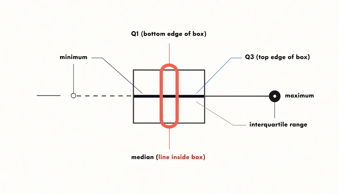
Because each of the five numbers has a clear statistical meaning, the resulting shape communicates dispersion, skew, and range in a compact space. A long upper whisker, for instance, suggests a stretched right tail, while a median line sitting close to one edge of the box hints at asymmetry within the middle half of the data. This economy of representation makes the box plot a natural first look at any numeric variable and a convenient building block when several distributions are placed side by side for comparison.
Box Plot
Learning to read these five summary numbers fluently is the foundation of effective data exploration. When the central median line sits closer to the bottom or top of the box, the distribution is skewed in that direction, which offers an early warning that a simple average may mislead. Because the interquartile range contains the middle fifty percent of observations, the box’s width tells you how tightly the bulk of the data clusters. A narrow box signals consistency, while a wide box indicates substantial spread among typical values.
The whiskers extend from the box toward the more extreme observations, usually stopping at the furthest point within one and a half times the interquartile range from each quartile. Points beyond the whiskers appear as individual markers and represent potential outliers. Treat these markers as prompts for investigation rather than verdicts: some reflect genuine extreme events worth understanding, others stem from data entry errors or measurement faults, and occasionally they arise naturally in heavy-tailed distributions. Comparing whisker lengths on either side of the box reveals asymmetry, since a long upper whisker paired with a long upper box half confirms right skew.
Practical reading habits help avoid mistakes:
- Always check the axis scale before judging distances, because a truncated axis exaggerates differences.
- Compare boxes across groups side by side to spot shifts in medians and changes in spread simultaneously.
- Note whether quartiles overlap between groups, since heavy overlap suggests the groups differ little in their central behavior.
With these habits, a single compact graphic yields a reliable picture of central tendency, variability, and the presence of unusual values.
Box Plot
The box plot’s great strength is its economy. Compressing a dataset into a single, legible glyph makes it possible to compare dozens of groups side by side without visual clutter, and the median line and interquartile range offer a robust picture of central tendency and spread that resists distortion by outliers. For audiences who need a quick read on where a distribution sits and how tightly it clusters, the box plot delivers that information with remarkable efficiency. It is also a standard tool with well-understood conventions, so its encoding is familiar to most analysts and requires little explanation.
That same economy carries a real risk: the box plot can hide the shape of the data. Because it summarizes only a handful of quantiles, it cannot reveal multimodality, skewness, or gaps. A bimodal distribution and a unimodal one can produce identical boxes if their quartiles and whiskers coincide, leaving the viewer with a false impression of homogeneity. Outliers are plotted as individual points, but their frequency and arrangement are not conveyed, and dense clusters of outliers may be mistaken for noise. The whiskers, often defined as 1.5 times the interquartile range, further compress the tails and can make heavy-tailed data appear tamer than it is.
These limits mean the box plot works best as a first-pass summary or as a complement to more detailed views. When the underlying distribution matters—when clusters, skew, or multiple modes could change the interpretation—the box plot should be paired with a method that shows the full shape, such as a histogram, density curve, or violin plot. Used alone, it offers a compact and robust overview; used without awareness of what it omits, it can smooth over exactly the features that drive decisions.
Violin Plot
The violin plot takes the skeleton of the box plot and dresses it with information about the full shape of the data. At its core lies kernel density estimation, a technique that places a small smooth bump at every observed data point and sums those bumps together to produce a continuous curve. The width of that curve at any given value reflects how densely observations cluster around it, so peaks indicate common values and narrow stretches indicate sparse regions. This estimated density is then mirrored on both sides of a central axis, producing the characteristic violin silhouette. Within or alongside that silhouette, the familiar box plot elements often remain: the median line, the quartile boundaries, and sometimes the whiskers, giving readers both summary statistics and distributional shape in a single view.
The practical payoff is that a violin plot reveals features the box plot cannot express, such as bimodality, skew, long tails, or subtle shoulders in the data. Two groups can share identical medians and quartiles while their violins look completely different, and that difference may carry the most important analytical insight. The bandwidth parameter of the kernel density estimator controls the smoothness of the outline, with wider bandwidths producing softer, more generalized curves and narrower bandwidths revealing finer local structure. Many implementations also vary the fill or trim the tails to avoid drawing density into regions where no data exist. By layering this continuous probability view over the standard five-number summary, the violin plot lets analysts see where values concentrate, how spread out they are, and what overall shape the distribution takes, all without leaving a single compact graphic.
Violin Plot
The violin plot’s distinctive shape is its primary interpretive tool: the width of the plot body at any given y-value represents the relative frequency or density of observations at that value. By tracing these swells and contractions along the vertical axis, you can read the distribution’s concentration directly. For example, a pronounced bulge near the median signals a large number of values in that range, whereas a thin neck indicates a sparse region. This visual encoding of frequency is what distinguishes the violin plot from simpler representations.
The symmetry of the violin (or lack thereof) further reveals skewness and multimodality. When the plot is split into two halves, each side can represent a different group, allowing direct comparison of densities. Interpreting the width requires attention to scale: the maximum width is typically normalized, so comparisons across violins of different sample sizes should be made with caution. Nonetheless, within a single violin, the swells are a reliable guide to where values concentrate. By learning to read these contours, analysts can quickly grasp central tendencies, dispersion, and the presence of outliers or gaps.
Violin Plot
Replacing the box with a mirrored density curve makes hidden structure apparent. When a dataset contains multimodal distributions, the violin swells in more than one place along its vertical axis, producing distinct bulges that correspond to separate concentrations of values. A bimodal split appears as two lobes separated by a narrow waist, immediately signaling that the observations likely come from two different subgroups rather than a single homogeneous population. These features remain invisible in a standard box plot, which cannot show where values cluster between the quartiles.
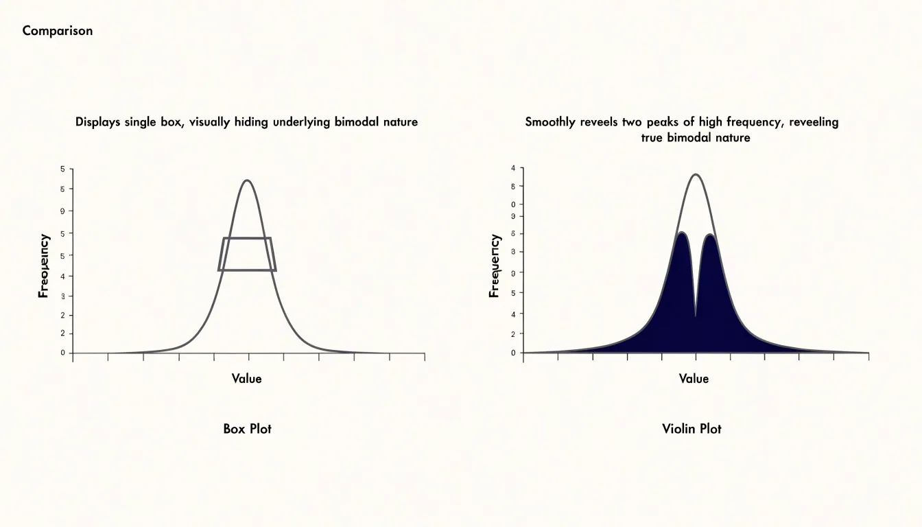
Groups that were not anticipated during data collection often surface in a violin plot. A small secondary bump near the top or bottom of an otherwise smooth curve can point to a handful of unusually high or low records, a distinct operating regime, or a separate measurement process mixed into the same column. Similarly, a shoulder on one side of the main peak suggests an overlapping cluster that is partially merged with the dominant one. Analysts reviewing many variables at once can scan a grid of violin plots and pick out the ones with irregular silhouettes, then investigate those variables further.
The density estimation underlying the violin also reveals skewness and tail behavior in a directly readable form. Long thin tails indicate rare extreme values, while flat, wide sections show where probability mass is spread evenly. Because the width at any height is proportional to the local density, the plot communicates how many observations sit at each value range without requiring a histogram bin choice.
For exploratory work, this shape-based view supports decisions about segmentation, outlier handling, and whether a single summary statistic is meaningful for a given variable. When a violin shows multiple peaks, reporting one median can obscure the very structure that matters most.
Box Plot vs Violin Plot
A side-by-side structural comparison highlights how the two charts encode the same space differently. Every element of a box plot is a line or a point, so the graphic communicates position and spread efficiently while leaving the interior of the distribution empty. A viewer can read the center and the middle fifty percent of the data at a glance, yet cannot tell whether the values cluster near the median, pile up at one tail, or form two separate humps. The violin plot occupies the same horizontal footprint and replaces the box and whiskers with a mirrored, smoothed outline. Many implementations draw a miniature box plot inside the violin, combining the density shape with the summary statistics in one figure.
Structurally, the box plot reduces a distribution to a handful of landmarks, while the violin plot reconstructs the full shape of the density curve. Both use a shared vertical axis for the measured variable, so multiple groups can be arranged side by side for comparison, and both are typically drawn with a categorical axis. The practical difference lies in information density: the box plot offers a compact, standardized encoding that is easy to scan across many groups, and the violin plot offers a richer picture of distribution shape at the cost of more visual detail and a smoothing parameter that influences the outline. Reading the two side by side shows how the same data set can yield a spare summary of quartiles and a full silhouette of density, with the internal box of a violin bridging the two representations.
Sample Size
When a dataset contains only a handful of observations, the violin plot’s kernel density estimate becomes unreliable. Because the curve sums smooth kernels placed around each data point, with five, ten, or even twenty observations the resulting shape reflects the chosen bandwidth as much as the underlying distribution. A narrow bandwidth produces a lumpy curve with spurious peaks at each observation, while a wide bandwidth over-smooths and can invent a unimodal silhouette that hides real gaps. Readers see an apparently precise, continuous shape and may infer structure that the data cannot support. Small samples also make the tails of the violin especially untrustworthy: kernel smoothing tends to extend density beyond the observed range, suggesting values that were never recorded.
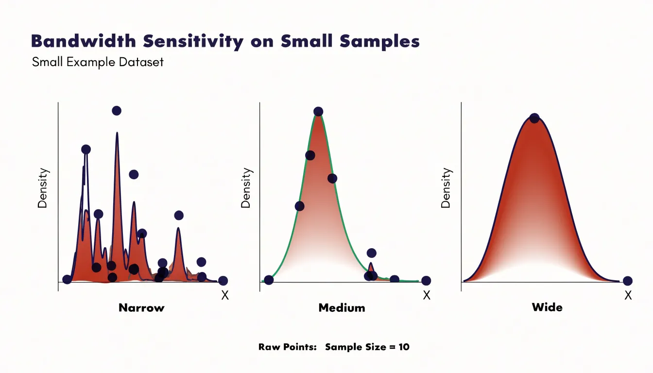
A box plot, by contrast, is built directly from order statistics. The median, quartiles, and whiskers are simple summaries of the observed values, requiring no smoothing or bandwidth choice. With a small sample the box plot may look sparse, and quartile estimates will wobble from sample to sample, but every element corresponds to an actual data point or an interpolated position between two of them. The interquartile range and median remain interpretable even with a dozen observations, and the whiskers honestly communicate the spread of what was measured. For an analyst working with limited data, the box plot therefore offers a more conservative and defensible summary, while the violin’s apparent richness of detail is an artifact of the estimation procedure rather than a property of the data itself.
Real World Example
Customer satisfaction surveys for essential oil blends typically produce ratings on a bounded scale, often one to five stars, gathered from hundreds or thousands of respondents. Each blend accumulates its own distribution of scores, and the shape of that distribution carries meaningful information. A lavender blend might average 4.2 stars, yet the underlying responses could cluster tightly around four, or split between enthusiastic fives and disappointed twos with little in between. These two scenarios share the same mean while telling very different stories about how customers actually experience the product.
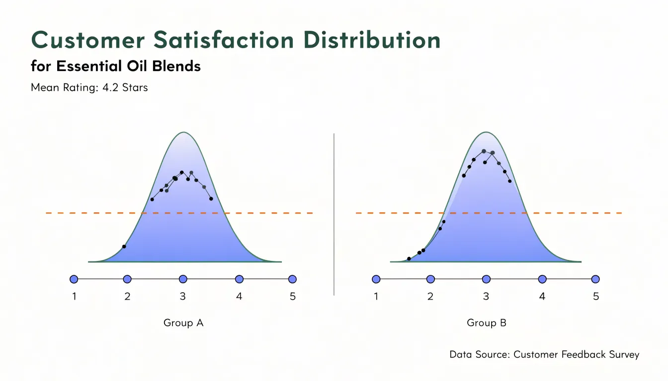
A box plot summarizing these survey scores gives a quick read on typical satisfaction and the spread of opinion. Analysts can compare blends side by side and immediately see which ones produce consistent ratings and which show wide dispersion. The box plot’s compact form works well for dashboards and executive summaries where dozens of blends need to be reviewed at once.
A violin plot exposes patterns a box plot can flatten out. A blend with a bimodal distribution, for instance, may have one segment of loyal repeat buyers rating it five stars and another segment of first-time users rating it two, perhaps because of scent expectations or price sensitivity. The violin shape makes that split visible, prompting follow-up questions about packaging, marketing claims, or the blend’s positioning.
Using both views together supports a practical workflow. The box plot handles rapid screening across a product line, and the violin plot invites closer inspection of blends whose distributions look unusual. Subtle perception trends, such as gradual shifts in the lower tail of ratings after a formulation change, become easier to detect and discuss with product teams.
Real World Example
Consider a specialty tea and spice retailer that sells three aromatic product blends across four seasons. The analytics team wants to understand both the central revenue each blend generates and how widely sales swing from quarter to quarter. To examine this, they collect two years of quarterly revenue figures for each blend and plot them side by side.
When the team builds box plots for each product line, the boxes and whiskers show where the middle half of each blend’s sales fall and the typical highs and lows, with any outlier quarters marked separately. For the chai blend, a box plot might show a compact box with a narrow spread, indicating steady revenue across seasons, while a spike in the winter quarter appears as a point beyond the upper whisker, capturing the holiday demand surge. The floral blend could show a much wider box, signaling inconsistent performance with some quarters producing strong revenue and others dragging.
The violin plots add density information on top of this summary. For the floral blend, the violin shape might be bimodal, with two bulges that correspond to a spring peak and a late-summer lull. That shape tells the team that the blend’s revenue clusters around two distinct seasonal levels rather than varying smoothly. For the chai blend, the violin would be wider near the median and taper toward the outlier, illustrating how concentrated most quarterly results are.
By comparing these visualizations, the retailer can decide which blends need seasonal marketing support and which hold steady on their own.
Choosing a Chart
Choosing between a box plot and a violin plot comes down to three practical considerations that guide most real-world charting decisions.
The first is the technical fluency of your audience. Box plots follow a compact, well-established grammar that most readers have encountered since secondary school: the median line, the quartile box, the whiskers, and the occasional outlier point. They require little explanation and can be dropped into a report or slide deck without a caption. Violin plots demand more interpretive work, since readers must understand kernel density estimation and learn to read the mirrored shape as a probability distribution. For a general business audience, this overhead often outweighs the extra detail a violin provides, while for a statistical or research audience the density view is familiar and welcome.
The second criterion is dataset size. With only a handful of observations per group, a box plot can be misleading, because quartiles and whiskers derived from ten or fifteen points are unstable and the picture looks more authoritative than the underlying data warrants. In that situation, showing individual points alongside the summary, or using a violin that makes the sparse data obvious, gives a more honest view. Large datasets flip the trade-off: box plots scale gracefully across dozens of groups, while violins become cluttered and slow to render.
The third criterion is distribution complexity. When distributions are symmetric, unimodal, and free of heavy outliers, the box plot captures nearly all the salient information with great economy. Multimodal or strongly skewed distributions are where the violin plot earns its place, because a box plot collapses bimodal data into a single median and interquartile range, hiding the structure entirely. Where such complexity matters to the argument or decision at hand, the violin plot tells the truer story.
Common Pitfalls
When working with violin plots, several common misinterpretations can distort the conclusions drawn from the visualization. A frequent error is to read the width of a violin at any given y-value as an absolute measure of volume. The width actually represents a kernel density estimate, which is scaled so that the total area under the curve equals one. This means that a wider section indicates a higher relative frequency of data points at that value, but it does not tell you how many observations are in that region. Comparing widths across violins of different sample sizes or across different variables can be misleading because the density is normalized. Always pair density plots with sample size information and avoid making claims about absolute counts from the width alone.
Another pitfall is ignoring the bandwidth used for kernel density smoothing. A small bandwidth produces a jagged shape that may reveal fine-grained structure but also noise, while a large bandwidth oversmooths and can hide important features such as multimodality. If you compare violins created with different bandwidths, differences in shape may be due to the smoothing parameter rather than the underlying data. To make valid comparisons, ensure that all violins in a single plot are generated with the same bandwidth and, ideally, report the bandwidth used.
Additionally, be cautious when interpreting the tails of the violin: kernel density estimates extend beyond the range of the data, so the apparent tails may not correspond to actual observations. Finally, remember that violin plots do not show the raw data points; they can obscure outliers and the exact sample size. Relying solely on the violin shape without overlaying a box plot, individual points, or summary statistics can lead to overlooking important data characteristics.
Tools and Libraries
Both box plots and violin plots are standard offerings in the major data visualization libraries for Python and R, which makes it straightforward to generate either chart with just a few lines of code:
- Seaborn (Python): Provides dedicated functions for each:
boxplot()andviolinplot()share a nearly identical interface, so you can switch between the two by changing a single function call while keeping the same dataset, grouping variables, and stylistic parameters. Seaborn’sviolinplot()also includes options to overlay a box plot or individual observations, combining the summary and distribution views in one figure. - Plotly (Python and R): Extends these capabilities to interactive web-based visuals. Its
graph_objectsmodule includesBoxandViolintrace types, and the higher-levelexpressAPI offerspx.box()andpx.violin()for quick exploration. Interactive features like hover tooltips, zooming, and toggling traces make Plotly particularly useful for dashboards and presentations where viewers may want to inspect individual data points. - ggplot2 (R): Takes a layered grammar-of-graphics approach. A box plot is built with
geom_boxplot(), and a violin plot withgeom_violin(); because both are geoms, they can be combined with the same mapping, faceting, and theming functions. This consistency means that switching between plot types requires only swapping the geom layer. For interactive R visuals, theplotlypackage can convertggplot2objects directly viaggplotly(), preserving the familiarggplot2syntax while adding interactivity.
Across all these tools, the key advantage is that the underlying data preparation remains the same. You can generate both plot types from a single data frame, compare them side by side, and choose the one that best communicates the distribution’s shape, central tendency, and variability for your audience.
Combining Charts
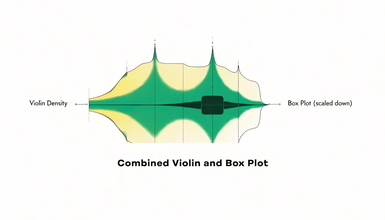
Combining charts through overlay is one of the most effective ways to get the strengths of two visualizations at once, and the pairing of a box plot nested inside a violin plot is a widely used example of this technique. The construction is straightforward: the violin silhouette is drawn first, showing the full estimated probability density of the distribution on each side of the central axis, and then a compact box plot is placed along that same axis within the violin body. The box plot is typically scaled down, sometimes to half width or less, so it reads as a clear visual anchor surrounded by the flowing density shape.
Decision Guide
A decision guide turns the comparison between box plots and violin plots into a practical routine you can apply to any dataset. Begin by naming the analytical question. If the goal is to compare medians and interquartile ranges across groups, or to flag outliers for follow-up, a box plot gives a compact and familiar summary that audiences read quickly. If the goal is to understand the full shape of each distribution, including multiple peaks, skew, or clustering near the tails, a violin plot exposes that structure.
A short flowchart can organize this choice:
- Ask whether sample sizes are large enough to estimate density reliably. Small groups can produce misleading violin shapes, while box plots remain stable summaries.
- Ask whether the audience needs a conventional summary or an exploratory view of distribution shape.
- Consider how many groups appear on the chart; dense comparisons often favor the visual economy of box plots, while a handful of groups leaves room for violins.
- Check whether outliers must remain individually visible, since a violin can obscure them unless overlaid with points or a box.
A companion checklist keeps the final decision grounded:
- Confirm the sample size per group.
- Note whether the distribution is unimodal or multimodal.
- Verify that axis scales are consistent across panels.
- Decide whether individual observations should be shown alongside the summary.
- Match the chart to the audience’s familiarity.
- Consider combining the two forms by embedding a box plot inside a violin.
Once these questions are answered in order, the choice becomes a repeatable step rather than a matter of preference.
Frequently Asked Questions
What do the five numbers in a box plot represent?
They are the minimum, first quartile, median, third quartile, and maximum. The box is drawn from Q1 to Q3 with the median line across it, and the whiskers extend toward more extreme observations.
How do I read the width of a violin plot?
The width at any y-value represents the relative frequency or density of observations at that value. A bulge signals many values in that range, while a thin neck indicates a sparse region, and the maximum width is typically normalized.
Are violin plots reliable with small sample sizes?
With only a handful of observations, the violin’s kernel density estimate becomes unreliable because the shape reflects the chosen bandwidth as much as the underlying data. A box plot is built from order statistics and remains interpretable with a small sample, though quartile estimates can wobble.
What is the difference between a box plot and a violin plot?
A box plot reduces a distribution to a handful of landmarks, while a violin plot reconstructs the full shape of the density curve with a mirrored, smoothed outline. Many violin implementations also draw a miniature box plot inside.
How do I choose between a box plot and a violin plot?
The article recommends considering audience technical fluency, dataset size, and distribution complexity. Box plots are compact and familiar for comparing medians and interquartile ranges, while violin plots expose full shape such as multimodality or skew.
What are common mistakes when interpreting violin plots?
A common mistake is reading violin width as an absolute count; width is a kernel density estimate scaled so the total area equals one, so it shows relative frequency. Comparisons can be misleading if sample sizes or bandwidths differ, and kernel density estimates extend beyond observed data, so pair violins with sample size information, box plots, points, or summary statistics.
Tony Astor
Tony writes about data visualization and the tools people use to build charts and dashboards. More about Data Illustrator