Box Plot: How to Read a Box and Whisker Chart
 By Tony Astor ·
Box Plot
A box plot (box-and-whisker plot) displays a dataset’s distribution using five summary statistics: minimum, first quartile (Q1), median, third quartile (Q3), and maximum. The box spans the interquartile range (IQR, Q3−Q1), containing the middle 50% of values, with a median line inside and whiskers extending to 1.5×IQR, beyond which points are plotted as outliers.
Table of Contents
Box Plot
A box plot, sometimes called a box-and-whisker plot, displays the distribution of a dataset through a small set of summary statistics. The central rectangle, or box, spans the interquartile range (IQR), running from the first quartile (Q1) at the 25th percentile to the third quartile (Q3) at the 75th percentile. This box contains the middle half of all observations, and its height or width gives an immediate reading of how tightly the central data cluster together. A line drawn across the box marks the median (the 50th percentile), and its position relative to the box edges reveals at a glance whether the middle section of data leans toward one end of the range.
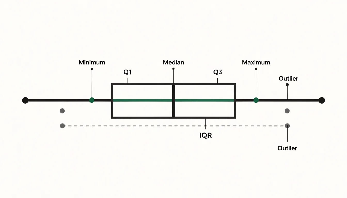
The whiskers extend outward from the box toward the minimum and maximum values that fall within a defined threshold, commonly 1.5 times the interquartile range beyond each quartile. These lines summarize the reach of the main body of data. Points lying beyond the whiskers are plotted individually as outliers, flagging observations that sit unusually far from the rest of the distribution.
The arrangement of these components makes the chart a fast diagnostic tool. When the median sits off-center within the box, or when one whisker stretches noticeably farther than the other, the shape signals skewness in the underlying data. A short box paired with long whiskers points to a concentrated center with wide tails, while a long box indicates broadly spread middle values. Comparing box plots across groups multiplies this value, since differences in medians, box lengths, and outlier patterns become visible side by side without any need to inspect raw values.
Five Number Summary
Five values define the structure of a box plot: the minimum, the first quartile (Q1), the median, the third quartile (Q3), and the maximum.
- Minimum: The smallest observation in the dataset.
- First quartile (Q1): The point below which roughly a quarter of the observations lie.
- Median: The center of the ordered data, with half the values falling below it and half above.
- Third quartile (Q3): The point below which roughly three-quarters of the observations lie.
- Maximum: The largest observation in the dataset.
The power of this summary lies in compression. Rather than displaying hundreds or thousands of raw values, five numbers preserve the essential profile of the distribution: where the data begins and ends, where its center rests, and how far the central bulk stretches. From these values alone, a reader can judge symmetry versus skew and compare the spacing between the minimum and Q1 against the spacing between Q3 and the maximum to see whether the tails are long or short.
Median Line
The median line inside the box marks the 50th percentile, dividing the dataset into two equal halves. It serves as a robust measure of central tendency, meaning it is largely unaffected by extreme values. Because it depends only on the rank order of observations, a handful of very large or very small values can shift the mean substantially while leaving the median unchanged.
Consider household income data, where a small number of extremely high earners pull the mean well above what a typical household earns. The median stays anchored near the middle of the distribution and gives a more faithful picture of the typical case.
This resilience makes the median particularly valuable when analyzing skewed data. In such distributions, the mean is dragged toward the tail and can misrepresent where most observations actually cluster. The median line remains in the dense part of the data, allowing readers to compare typical values across several boxes even when those groups have different spreads, outliers, or asymmetries.
Interquartile Range
The interquartile range (IQR), computed as Q3 - Q1, is represented by the span of the main box and encloses the middle 50 percent of all data points. If you lined up every observation from smallest to largest and split the data into four equal groups, the box would cover the second and third groups, leaving the lowest quarter below the bottom edge and the highest quarter above the top edge.
The IQR measures variability in the central portion of the data. Because the calculation depends only on quartiles, the IQR stays stable in the presence of extreme values. A single unusually large or small observation can stretch the overall range dramatically, yet it leaves the quartile boundaries essentially untouched. This stability makes the IQR a dependable summary of spread for skewed distributions and datasets containing outliers.
Quartiles
Quartiles are the three boundary values (Q1, Q2, and Q3) that divide an ordered dataset into four segments of equal size, each containing roughly 25 percent of the observations. Different software packages handle the interpolation details for computing quartiles slightly differently, yet the underlying principle stays the same.
Interpreting quartiles goes beyond naming three numbers. The distances between Q1 and Q2 (the median), between Q2 and Q3, and between the extremes and the adjacent quartiles reveal how densely observations cluster in each quarter of the distribution. A short span holding 25 percent of the points signals a dense concentration of values, while a wide span covering the same share indicates that the data are spread thinly across that region. Comparing the gap from Q1 to Q2 with the gap from Q2 to Q3 shows which half of the central data is more compressed, indicating whether the distribution leans toward lower or higher values.
Whiskers
The whiskers extending from both ends of the box communicate how far the data spread beyond the middle quartiles. Each whisker typically extends to the most extreme data point that still falls within 1.5 times the IQR from the nearest edge of the box:
- Upper whisker: Reaches to the largest observation no farther than 1.5 × IQR above Q3.
- Lower whisker: Reaches to the smallest observation no farther than 1.5 × IQR below Q1.
This 1.5 × IQR threshold is a standard convention, though some software packages allow it to be adjusted or offer alternatives such as drawing whiskers to the absolute minimum and maximum values or to specified percentiles.
Because standard whiskers stop at the last non-outlier data point rather than stretching to the absolute extremes, they mark the boundary of the typical range of the data. A long whisker signals a gradual spread of values away from the middle half, while a short whisker suggests that the data drop off quickly beyond the quartiles.
Outliers
Outliers are individual data points that fall unusually far from the rest of a distribution, plotted as separate markers beyond the whiskers. These isolated points may represent genuine but rare events—such as an exceptional sale price or an unusually large measurement in a scientific sample—or they may signal a recording mistake, a transcription error, or a faulty instrument reading.
Visualizing outliers relies on thresholds built from the IQR:
- Mild outliers: Points lying between 1.5 and 3 times the IQR from the box, commonly shown with open circles.
- Extreme outliers: Points lying beyond 3 times the IQR from the box, often shown with asterisks or filled markers.
Reading these markers involves checking how many outliers appear, how far they lie from the whiskers, and whether they cluster on one side of the box. A single distant point suggests a possible error or a one-off anomaly. Several points stretching in the same direction may indicate a skewed distribution rather than simple mistakes, helping analysts decide whether to investigate, correct, or retain the unusual observations.
Side by Side Box Plots
Side by side box plots arrange several box-and-whisker diagrams along a shared axis so that distributions from different categories or experimental groups can be compared on a common scale. The technique is common in experimental work, where each box may represent a treatment group, a time point, or a demographic category, and in quality control, where boxes track variation across production lines or suppliers.
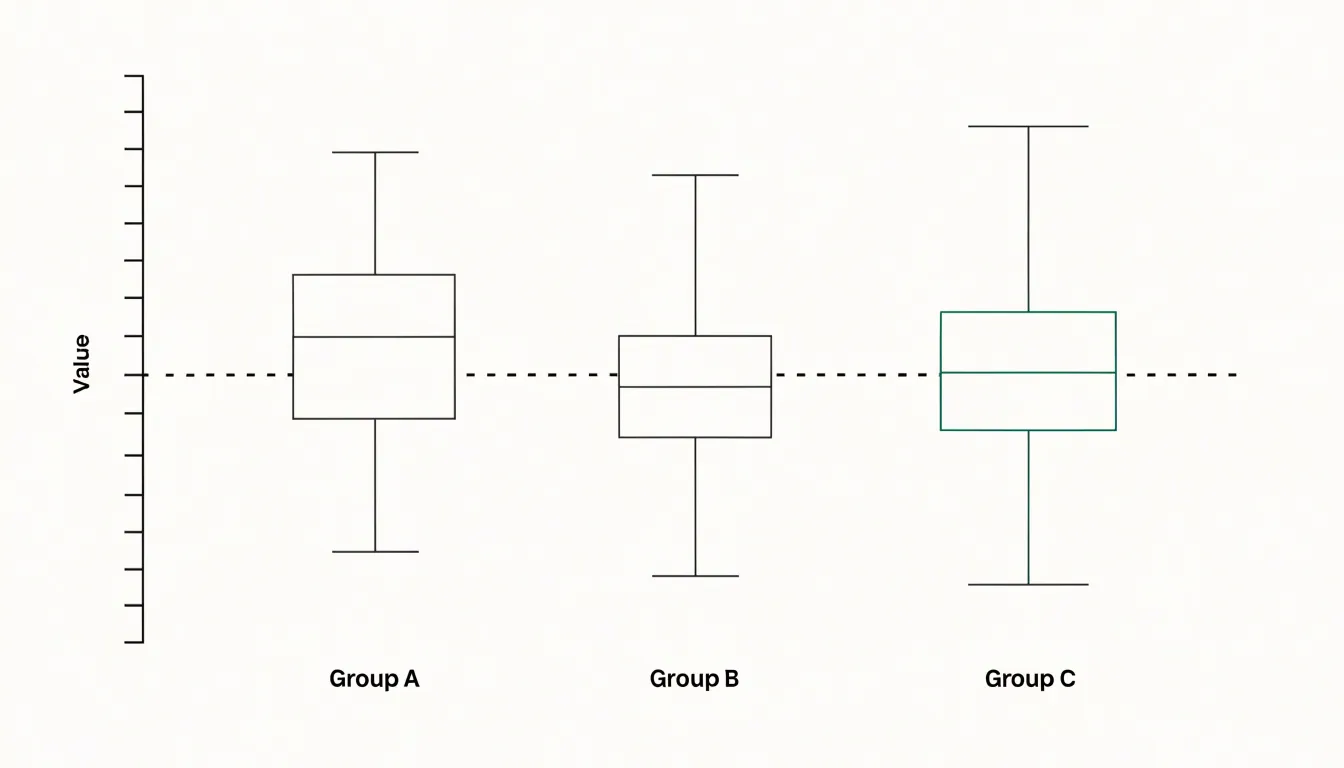
Tracing an imaginary line across the medians shows whether one group tends to sit higher or lower than the others, while box heights compare internal variability. Overlap between boxes carries important information:
- Minimal overlap: The groups likely differ in a meaningful way, since most of the central mass of each distribution occupies distinct regions of the scale.
- Heavy overlap: The groups resemble one another, and any difference in medians may be small relative to the natural variability within each group.
Comparing whiskers and outlier patterns adds nuance, revealing cases where medians coincide but one group has a much longer tail. Ordering the boxes by median or by category label, keeping axes consistent, and labeling groups clearly all improve readability.
Skewed vs Symmetric Data
The lengths of the whiskers and the position of the median line inside the box diagnose a distribution’s shape:
- Symmetric data: The median sits close to the center of the box (the distance from Q1 to the median roughly equals the distance from the median to Q3), and the whiskers are of comparable length on both sides.
- Right-skewed (positively skewed) data: The median sits nearer Q1 and the upper whisker stretches noticeably farther than the lower one. Most observations cluster at the low end, while a long upper tail of larger values pulls the upper whisker outward.
- Left-skewed (negatively skewed) data: The median sits closer to Q3 with a longer lower whisker, as a tail of unusually small values extends downward.
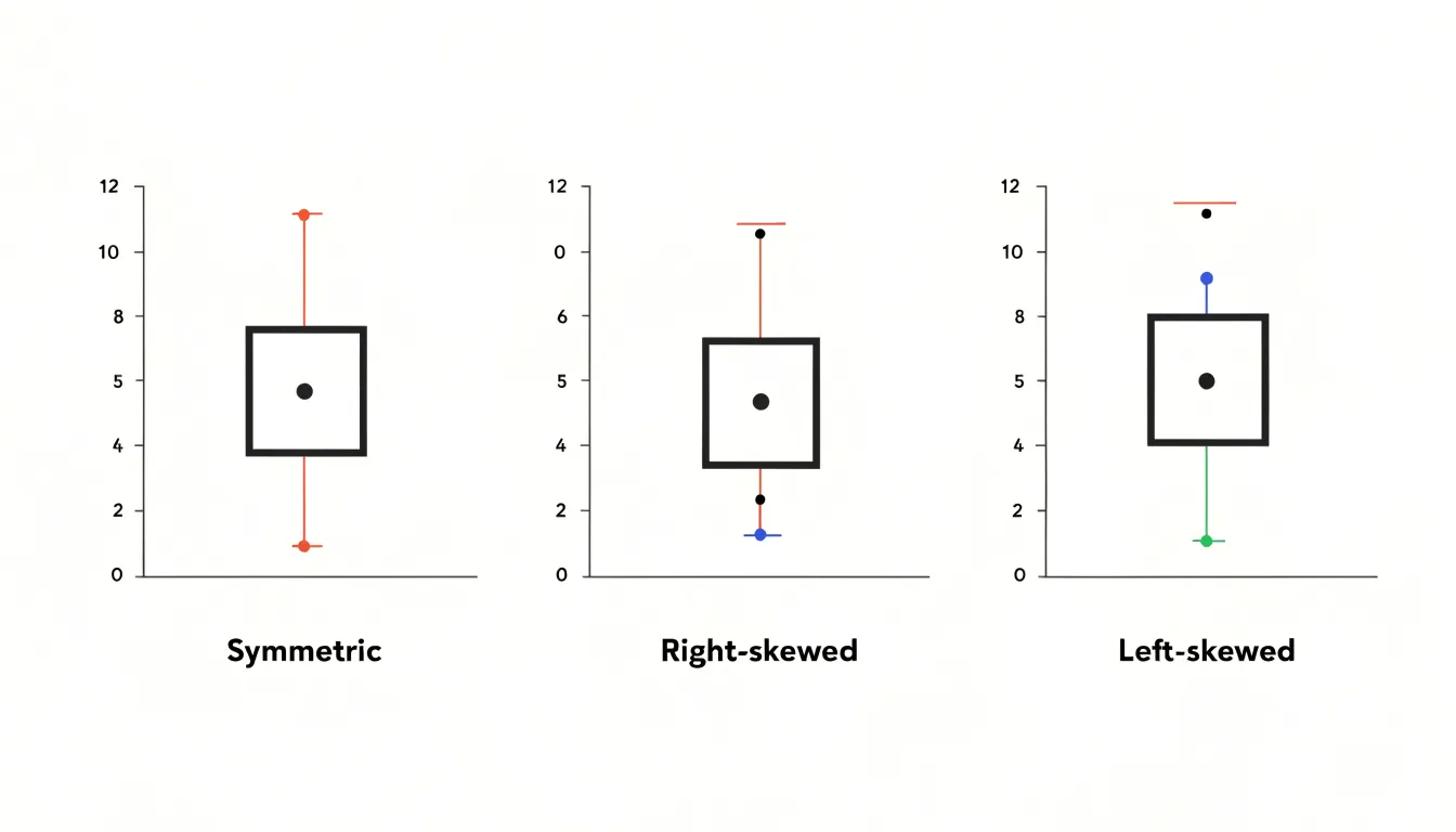
A practical habit is to compare the distances from the minimum to Q1, from Q1 to the median, from the median to Q3, and from Q3 to the maximum. In a symmetric dataset, these segments are broadly similar in scale. Large discrepancies point to asymmetry even before any numerical skewness measure is calculated. Note whether the box itself is lopsided, since an off-center median inside an otherwise balanced plot can still reveal mild skew in the central half of the data.
Box Plots vs Histograms
Choosing between a box plot and a histogram depends on dataset size and the questions the visualization is meant to answer.
Because a box plot condenses a distribution into five summary values and outliers, it occupies very little space and scales gracefully across numerous categories. An analyst comparing test scores across classrooms, sales figures across regions, or response times across servers can place many box plots along a shared axis. When the dataset is large, the five-number summary remains stable; for small datasets, it works as a concise portrait, though each quartile may rest on only a handful of points.
The trade-off is that a box plot hides the internal shape of the distribution. Two datasets with identical five-number summaries can have very different underlying forms, and the box plot will not reveal whether the data are unimodal, bimodal, or heavily clustered.
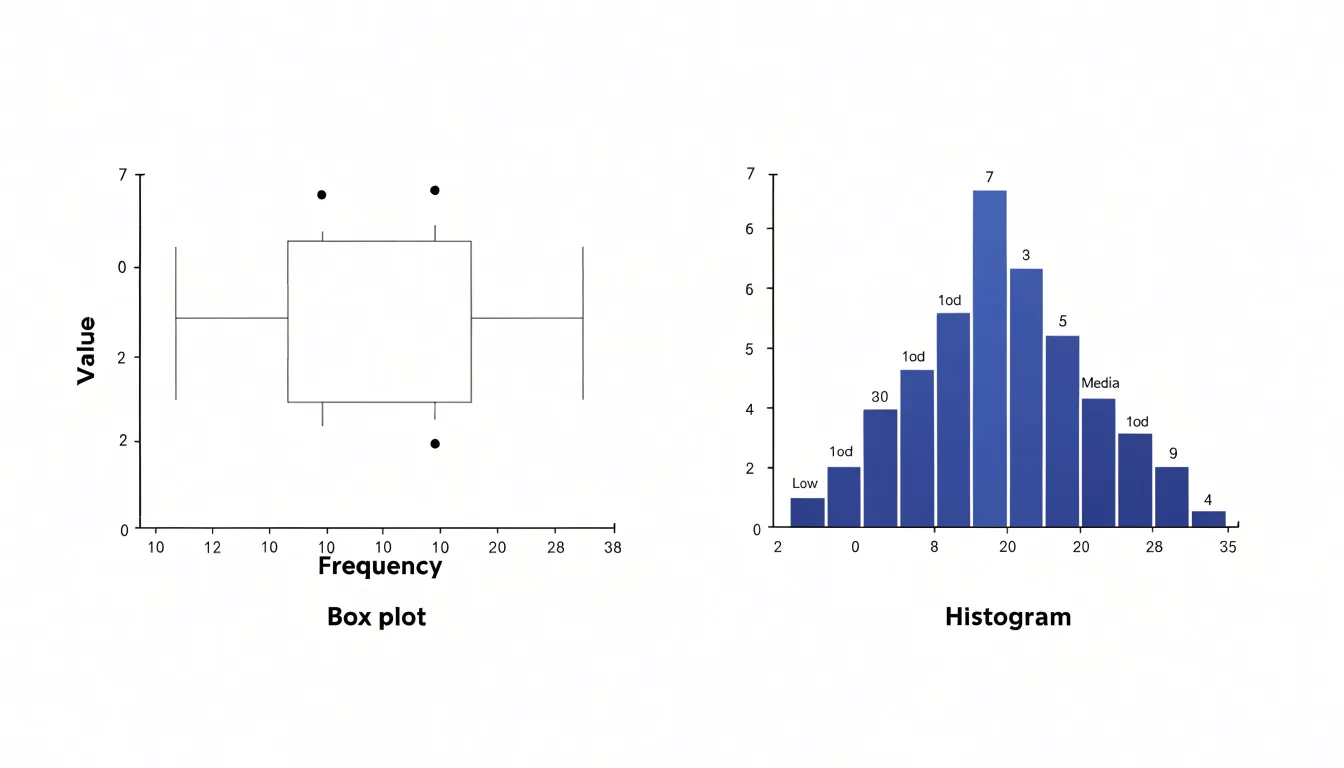
A histogram addresses that gap by binning observations and drawing bars whose heights show frequency. The resulting silhouette exposes modality, gaps, and the smoothness or lumpiness of the distribution, making it the better choice for understanding the internal structure of a single dataset. However, histograms need enough observations to populate the bins meaningfully; with very small samples, the bars become erratic and depend heavily on bin width. In practice, box plots serve comparison across groups, while histograms serve diagnosis of shape within a group, and the two frequently appear together.
Calculating Quartiles and IQR
To find Q1, Q3, and the IQR by hand, start by ordering your data from smallest to largest. The median of the entire dataset (Q2) splits the values into a lower half and an upper half. If the number of values is odd, exclude the median itself when forming the two halves. Q1 is the median of the lower half, and Q3 is the median of the upper half.
For example, take the nine values 3, 5, 7, 8, 10, 12, 14, 15, 20:
- The overall median (Q2) is
10. - Exclude
10to form the lower half (3, 5, 7, 8) and the upper half (12, 14, 15, 20). - Find the median of the lower half: (5 + 7) / 2 = 6, so Q1 = 6.
- Find the median of the upper half: (14 + 15) / 2 = 14.5, so Q3 = 14.5.
- Subtract Q1 from Q3 to get the interquartile range: IQR = 14.5 - 6 = 8.5.
When datasets are large, spreadsheets and statistical software handle the ordering and locating of quartile positions, but the underlying arithmetic remains the same.
Drawing Whiskers and Detecting Extremes
When constructing a box plot, whisker length is governed by statistical boundaries called fences:
- Calculate the step value by multiplying the IQR by 1.5 (Step = 1.5 × IQR).
- Find the upper fence by adding the step to the third quartile (Q3 + Step).
- Find the lower fence by subtracting the step from the first quartile (Q1 - Step).
- Draw the upper whisker from the top edge of the box to the largest actual data value that does not exceed the upper fence.
- Draw the lower whisker from the bottom edge of the box to the smallest actual data value that remains at or above the lower fence.
- Plot any value lying beyond either fence individually as an outlier marker.
Because whiskers end at actual observed data points rather than at the calculated fences themselves, they stay anchored to real measurements in the dataset. Computing both fences and sorting the data beforehand allows whisker endpoints and outliers to be located and placed accurately on the scale.
Common Reading Mistakes
Whisker length is one of the most frequently misread features of a box plot because the eye naturally equates visual length with quantity. A long whisker looks heavier, as though it carries a larger share of the observations, while a short whisker appears sparsely populated.
This intuition misleads. Whisker length shows dispersion—the distance the data travel in the units of the variable—rather than density, the concentration of points in that region. Each of the four regions defined by the quartiles and the extremes contains approximately 25 percent of the data, regardless of how wide or narrow they appear on the page. A compact box holds 50 percent of the observations, while a stretched whisker holds at most 25 percent.
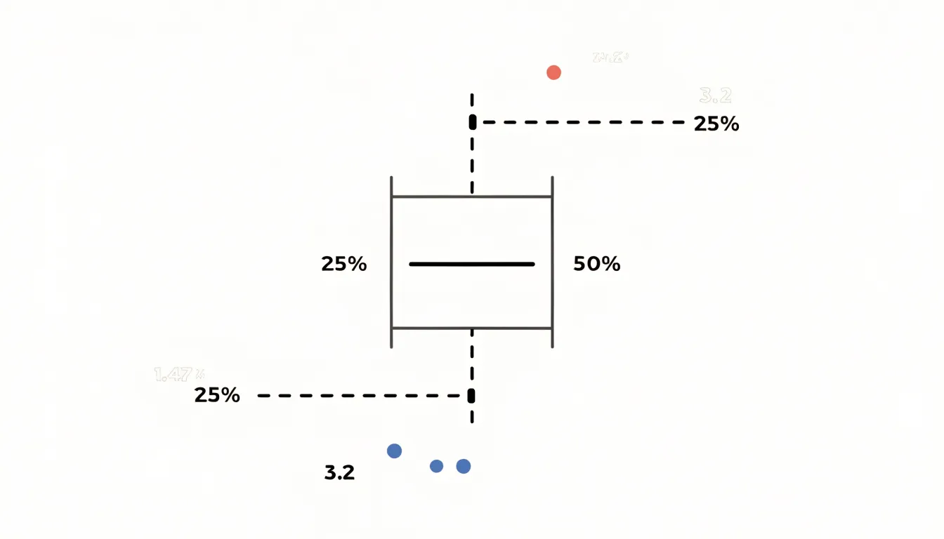
Skewed distributions routinely produce one whisker much longer than the other, and the longer side simply contains values spread thinly over a wider range. Keeping this quartile logic in mind prevents visual length from driving unsupported conclusions about sample size or point density.
Real World Examples
Box plots are widely used across industries to monitor distributions and spot anomalies:
- Finance: Analysts compare the spread of returns across investment portfolios or track monthly spending patterns. A box plot of transaction amounts reveals the median purchase size, the range where most activity falls, and any unusually large transfers sitting outside the whiskers.
- Healthcare: Administrators and clinicians compare lab results, quality-of-care metrics, and patient wait times across departments or facilities. Plotting blood pressure readings for patient groups side by side shows which group has a wider spread and which individual readings are statistical outliers worth a second look.
- E-commerce: Teams monitor order values, delivery times, and conversion rates across regions or product categories. A sudden lengthening of the upper whisker on a delivery-time plot signals growing process variability before customers complain.
- Operations and Manufacturing: Business analysts chart manufacturing lines, call centers, or payment pipelines so the typical range of performance is obvious and any point beyond the whiskers stands out for investigation.
Overview
Reading a box plot fluently follows a four-step sequence from center to extremes:
- Locate the median line: Note the midpoint of the dataset and where it sits relative to the box edges to check for symmetry or skew.
- Survey the box (IQR): Check the distance between Q1 and Q3 to judge how tightly or widely the middle 50 percent of typical values cluster.
- Examine the whiskers: Compare the lengths of the upper and lower tails to see the reach of typical values and confirm any skewness hinted at by the median.
- Inspect the outliers: Count the individual points beyond the whiskers and note how far they lie from the rest of the distribution to spot potential errors or rare events.
Frequently Asked Questions
What does a box plot show?
A box plot displays the distribution of a dataset using summary statistics. The box spans the interquartile range from Q1 to Q3, the median line marks the 50th percentile, and the whiskers and outlier markers summarize the rest of the distribution.
What five numbers are used in a box plot?
The five-number summary consists of the minimum, first quartile (Q1), median, third quartile (Q3), and maximum. These values show where the data begin and end, where the center rests, and how far the central bulk stretches.
Why is the median line useful when data are skewed?
The median line marks the 50th percentile and is a robust measure of central tendency that is largely unaffected by extreme values. In skewed data, the mean can be dragged toward the tail, while the median remains in the dense part of the data.
How is the interquartile range calculated and what does it represent?
The interquartile range is calculated as Q3 minus Q1. It is represented by the span of the main box and encloses the middle 50 percent of all data points.
How far do box plot whiskers extend?
Whiskers typically extend to the most extreme data point that still falls within 1.5 times the IQR from the nearest edge of the box. Points beyond the whiskers are plotted individually as outliers.
How can you tell if data are skewed from a box plot?
In right-skewed data, the median sits nearer Q1 and the upper whisker stretches farther than the lower one. In left-skewed data, the median sits closer to Q3 with a longer lower whisker, while symmetric data have a median near the center of the box and comparable whisker lengths.
Tony Astor
Tony writes about data visualization and the tools people use to build charts and dashboards. More about Data Illustrator