Best Data Visualization Tools Compared
 By Tony Astor ·

Best Data Visualization Tools Compared
Bar charts compare discrete categories using bar length, line charts show change over continuous time, and pie charts show part-to-whole shares for small datasets. Scatter plots reveal correlations, clusters, and outliers, while heatmaps encode magnitude by color across two dimensions. Histograms show distributions, area charts emphasize cumulative volume, treemaps nest hierarchies, and waterfall charts decompose change.
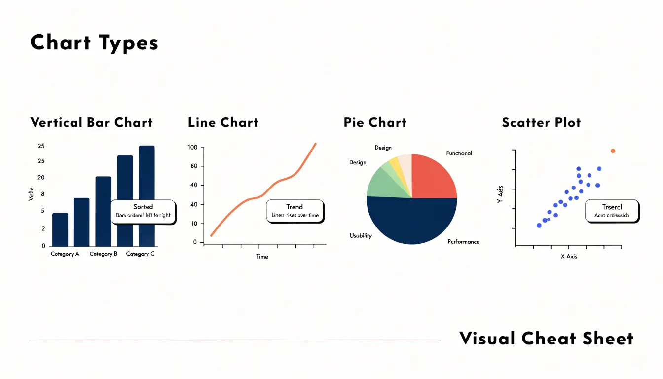
Table of Contents
Chart Type
Bar charts remain the workhorse for comparing values across discrete categories, whether you are ranking product lines, survey responses, or regional sales figures. Each bar represents a single category, and its length encodes the value, so readers can compare magnitudes without decoding complex legends. The choice between vertical and horizontal orientation depends on your labels. Vertical bars suit short category names such as months or quarters, while horizontal bars accommodate longer labels like department names or survey questions, since the text can run left to right without rotation or truncation. Horizontal orientation also keeps long labels readable on narrow screens and in printed reports.
Sorting is one of the most consequential design decisions. Alphabetical order helps readers locate a specific category, but it buries the comparative ranking. Sorting bars by value, either descending or ascending, immediately shows which category leads and which trails. Reserve alphabetical or logical sequences such as months for cases where readers already expect that order. If one category deserves emphasis, use a single contrasting color while keeping the rest neutral.
Spacing affects how easily the eye groups and separates bars. Keep the gap between bars consistent and noticeably narrower than the bars themselves; a common guideline is roughly half the bar width. Wider gaps fragment the visual comparison, while bars that touch read as a histogram rather than a category chart. Start the value axis at zero for bar charts, since bar length carries the meaning and a truncated axis distorts the comparison. Limit the number of categories to what a reader can scan comfortably, grouping minor categories into an ‘Other’ bar when necessary.
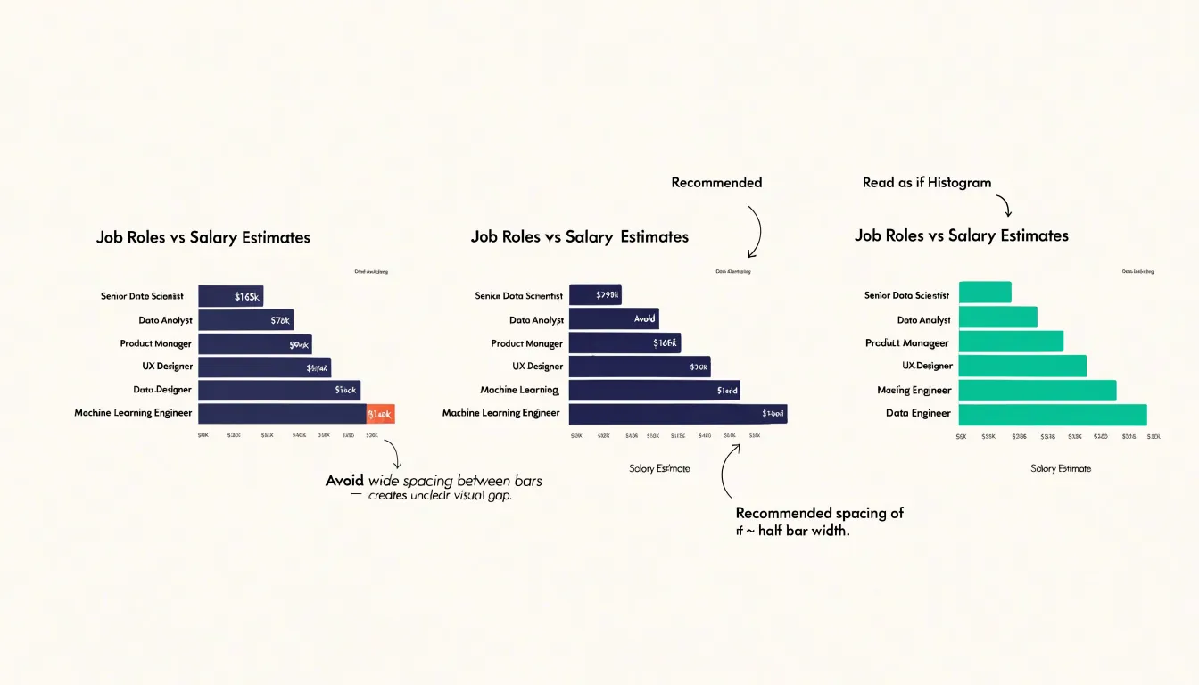
Chart Type
Line charts are the natural choice for showing change across a continuous span of time, such as daily website traffic, monthly revenue, temperature readings, or sensor output. Because the data points are joined by a line, the viewer can easily perceive the direction and speed of movement: a rising line communicates growth, a flattening line signals a plateau, and a steep drop draws the eye immediately.
The connected data points also reveal seasonal patterns—regular peaks and troughs, weekly cycles, or annual fluctuations—helping analysts distinguish recurring behavior from one-off anomalies. Viewers can judge the long-term trajectory while still noticing short-term variation. When building a line chart, keep the time axis evenly spaced and ordered, avoid plotting too many series at once, and label the axis clearly to preserve the sense of continuity.
Chart Type
Pie charts show how individual pieces contribute to a total, mapping each category to a slice whose angle is proportional to its share of the whole. They work best for dashboards, executive summaries, and reports where the dataset is small and the central question is a straightforward part-to-whole comparison, such as whether one segment dominates or the parts are roughly balanced.
Human perception can judge whether one slice is larger than another when the difference is pronounced, but accuracy drops quickly as slices multiply and their angles converge. Limit a pie chart to five or six categories at most to keep each slice large enough to compare and labels readable. Too many thin wedges create a ring of slivers with overlapping callouts or noisy legends. When a dataset includes many small categories, group the least significant ones into a combined ‘other’ slice, and use consistent ordering and restrained color.
Chart Type
Scatter plots explore the relationships between paired numerical variables by placing one variable along the horizontal axis and another along the vertical axis. Each point represents a single observation, revealing correlations at a glance: a tight diagonal band of points signals a strong linear relationship, while a diffuse cloud suggests little or no association.
Beyond correlation, scatter plots expose clusters and outliers:
- Clusters: When observations group into distinct regions, they often point to meaningful subpopulations, such as customer segments, geographic regions, or experimental conditions. Analysts can color or size the markers by a third variable to layer additional context onto the chart.
- Outliers: Because scatter plots preserve every individual data point rather than aggregating them into an average, points sitting far from the main concentration stand out clearly. This flags data entry errors, rare events, or genuinely unusual cases during early data quality checks.
Most data visualization tools implement scatter plots with options for trend lines, marker transparency to handle overplotting, and interactive tooltips that reveal exact values in large, dense datasets.
Chart Type
Heatmaps turn dense, multidimensional data into a color-coded matrix where shade intensity conveys magnitude. Each cell represents the intersection of two dimensions—such as day of week against hour of day, or product category against region—while its color encodes a third value like session count, revenue, or error rate.
High-value combinations render as deep, saturated cells, while low-activity combinations fade into pale or neutral tones. This makes heatmaps effective for identifying hot spots (such as peak traffic windows, best-selling store locations, or clusters of support tickets) and anomalies (an unexpectedly dark cell in a quiet row, or a light cell inside a strong band). Because the entire matrix fits in a single view, a grid of hundreds of cells remains readable where overlapping line series would become cluttered.
Visualization tools typically offer sequential color palettes for single-direction metrics and diverging palettes for values that move above and below a baseline, such as variance from target. Keep the color scale perceptually uniform, label the axes, and include a legend so readers can translate hue back into numbers.
Chart Type
Histograms show how a continuous quantitative variable is distributed across its range. The chart divides the full span of observed values into adjacent bins and counts how many observations fall into each one. The resulting bars are plotted side by side with no gaps. Because the horizontal axis represents a continuous scale, the width and number of bins chosen directly influence the visible shape of the data.
A histogram surfaces several distribution properties at once:
- Central tendency: The region where the tallest bars cluster, showing where typical values lie.
- Spread and variance: How widely the observations fan out across the axis.
- Skewness: Asymmetry in the profile, where a long tail to the right indicates positive skew and a tail to the left signals negative skew.
- Modality and gaps: Multiple peaks suggest mixed populations within a dataset, while gaps or isolated bars point to outliers, impossible values, or suspicious clustering.
These insights guide practical analytical decisions. Heavily skewed data may call for median and interquartile range rather than mean and standard deviation, or indicate that a variable needs transformation before modeling. Analysts can also compare histograms across groups or time periods to see how distributions shift.
Chart Type
Area charts fill the space beneath a line graph to emphasize volume and accumulated value rather than just direction of change. This makes them a natural fit for cumulative totals and running sums—such as monthly revenue, registered users, or total hours logged—where the total at any point in time matters.
Stacked area charts layer multiple series on top of one another so the combined height represents an overall total while individual bands show how each component contributes over time, such as different product lines adding to overall sales. To keep the chart readable, use a subtle fill, gradient, or transparency so the underlying gridlines and axis labels remain visible. Use area charts to communicate scale and accumulation over time rather than precise point-to-point comparisons.
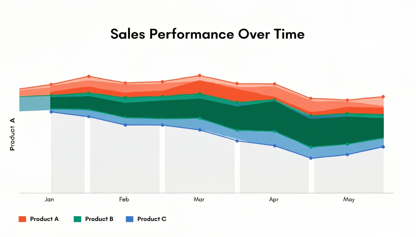
Chart Type
Treemaps visualize hierarchical data using nested rectangles whose areas are proportional to a quantitative value. A viewer can read both the structure of the hierarchy (through how child rectangles tile their parent rectangle’s area) and the relative magnitude of each category (through rectangle size). A common convention colors rectangles by parent group or by a separate measure to reinforce the hierarchy across levels.
Compared with bar charts, treemaps trade precise length comparisons for compact space efficiency, scaling to large numbers of categories without the empty regions that affect multi-slice pie charts. Because the smallest rectangles in deep hierarchies are difficult to label, many tools add tooltips or zoom-and-drill interactions. When comparing visualization tools, check whether they support multi-level nesting, separate color encoding, readable labeling, and interactive exploration of smaller nodes.
Chart Type
Waterfall charts show how a starting value moves to a final value through a series of intermediate additions and subtractions. The first bar shows the opening figure, such as last quarter’s revenue or a starting headcount budget. Subsequent bars float between the baseline and the running total, with upward steps marking gains and downward steps marking losses, connected by lines that trace the cumulative flow. A final bar anchored to the axis lands on the closing figure.
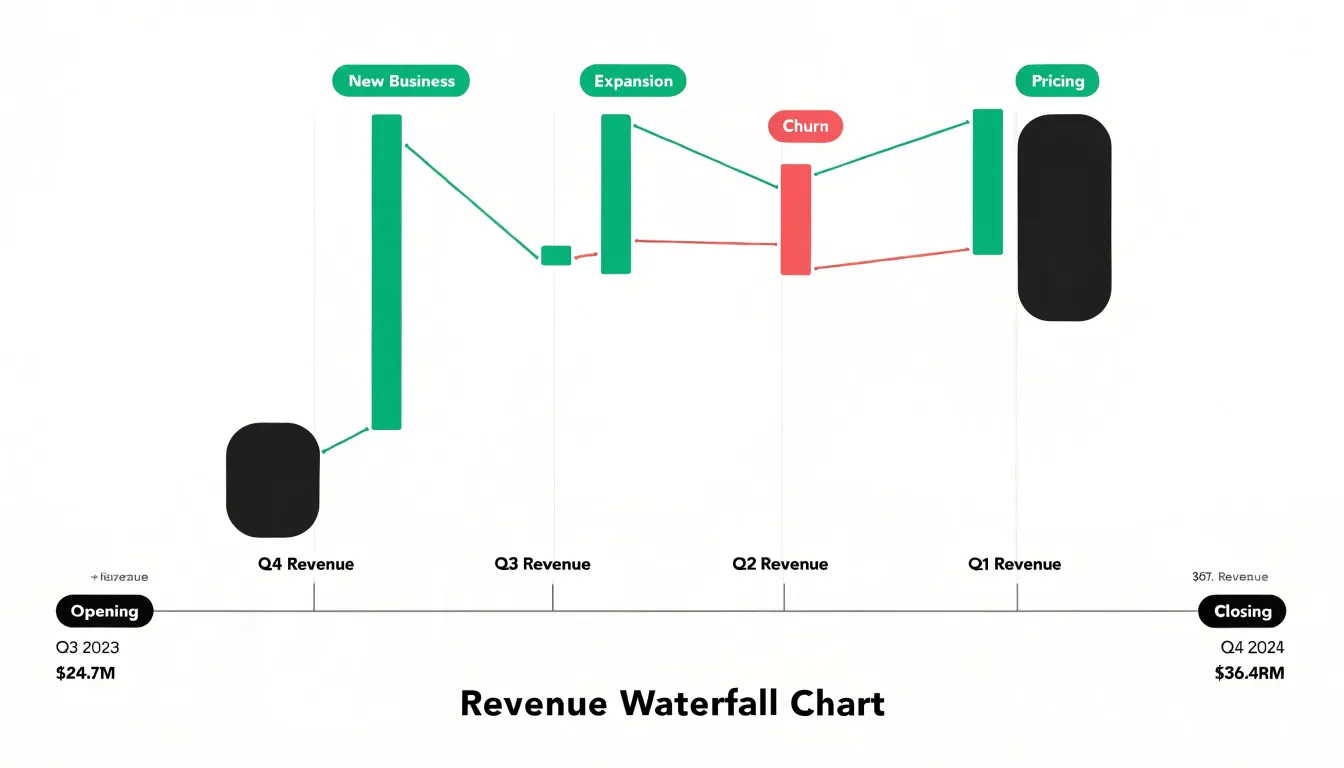
This format is built for decomposing variance rather than showing absolute metric levels:
- Sales reports: Breaking a quarterly revenue shift into new business, expansion, churn, and pricing effects.
- Finance reviews: Decomposing a margin change into input costs, labor, and overhead.
- Project updates: Showing budget movement as individual approvals and overruns.
Because each bar is discrete, it can carry short labels or commentary explaining what drove each step of the change.
Chart Type
Funnel charts visualize sequential processes where a population moves through mutually exclusive stages, such as sales pipelines, user onboarding flows, or e-commerce checkouts. Each stage is represented as a horizontal bar or vertical stack sized proportionally to the remaining entities, making progressive attrition immediately visible.
Comparing conversion rates between stages spotlights specific friction points—for example, showing that users abandon their carts at the shipping cost disclosure step. The overall shape also diagnoses pipeline health: a steep early drop-off suggests problems with initial engagement or lead quality, while a gradual decline indicates a healthier process. Funnel charts often include annotations or secondary bars showing stage-to-stage conversion percentages or time spent at each stage, provided the underlying data is accurately segmented.
Chart Type
Gantt charts map project schedules by depicting each task as a horizontal bar spanning its start and end dates along a timeline. This layout shows task sequences, durations, overlaps, and schedule gaps in a single view.
- Dependencies: Arrows connecting bars indicate which tasks must finish before others can begin.
- Milestones: Diamonds or flags mark critical phases or deliverables against key deadlines.
- Resource allocations: Bar colors or labels show which team members or equipment are assigned to each task and when they are occupied.
Project teams use Gantt charts to spot bottlenecks, adjust schedules, and coordinate timelines across stakeholders.
Chart Type
Dashboard layouts combine complementary charts on a single screen so viewers can move from a summary metric to supporting context without switching tabs. For example, a line chart tracking national performance over time pairs naturally with a bar chart comparing regional totals and a heatmap showing activity clusters.
Layout discipline keeps multi-panel views coherent:
- Consistent encoding: Shared date ranges, aligned axes, and uniform color coding across panels let viewers compare charts without mental conversion.
- Logical zoning: Grouping related metrics into distinct zones—such as revenue on one side and customer activity on the other—establishes a predictable visual structure.
- Whitespace and titles: Clear panel titles and adequate spacing prevent crowding.
When executives review the same dashboard layout regularly, familiarity with the arrangement makes regional dips or emerging anomalies stand out immediately.
Chart Type
KPI cards highlight a single key metric—such as customer acquisition cost, monthly active users, or average order value—as a prominent standalone number. Positioned in small groups at the top of a dashboard, they give viewers an instant summary of top-priority goals before they explore detailed charts below.
Because a bare number like 4,280 carries little meaning on its own, an effective KPI card pairs the headline figure with contextual indicators: a comparison to the previous period, a target threshold, a percentage change, a color-coded status arrow (such as a green upward arrow for a 14% quarterly revenue increase), or an embedded sparkline. Limit the number of KPI cards on a dashboard so the critical figures retain their visual prominence.
Chart Type
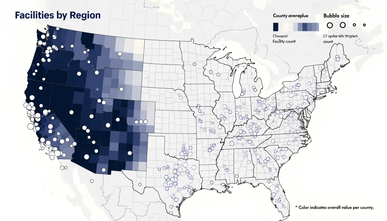
Geographic maps display location-based data across physical territories, primarily using two formats:
- Choropleth maps: Regions such as states, counties, or postal districts are filled with graduated colors to show where values sit above or below a threshold, revealing spatial patterns like border clusters or interior corridors. Choropleths work best with normalized values (rates or percentages), because raw counts usually just reflect population size. They suit comparisons across administrative boundaries used for budgets or policy.
- Bubble maps: Symbols are placed at specific coordinates—such as store locations, incidents, or customer addresses—and scaled in diameter to the value they represent. Because bubbles plot independently, dense urban corridors can show overlapping magnitudes that a filled polygon map would flatten into a single color.
Used together, the two formats can cross-check a geographic pattern: a choropleth might highlight elevated rates in several counties, while overlaid bubbles reveal whether those rates concentrate in a few specific facilities or spread evenly across the region.
Frequently Asked Questions
When should I use a bar chart instead of a line chart?
Use bar charts for comparing values across discrete categories, and line charts for showing change across a continuous span of time. For bar charts, start the value axis at zero because bar length carries the meaning.
How many slices should a pie chart have?
Limit a pie chart to five or six categories at most so each slice stays large enough to compare and labels remain readable. When a dataset includes many small categories, group the least significant ones into a combined “other” slice.
What is the difference between a histogram and a bar chart?
Bar charts compare values across discrete categories using separated bars, while histograms show how a continuous quantitative variable is distributed across adjacent bins with no gaps. In a histogram, the width and number of bins chosen directly influence the visible shape of the data.
What can a scatter plot reveal about my data?
Scatter plots explore relationships between paired numerical variables and can reveal correlations, clusters, and outliers. Because they preserve every individual data point, outliers stand out clearly during early data quality checks.
How can I make a dashboard layout easier to read?
Use consistent encoding across panels, such as shared date ranges, aligned axes, and uniform color coding, and group related metrics into logical zones. Clear panel titles and adequate spacing also help prevent crowding.
When should I use a choropleth map instead of a bubble map?
Choropleth maps fill regions with graduated colors to show where values sit above or below a threshold, and they work best with normalized values such as rates or percentages. Bubble maps place scaled symbols at specific coordinates, which can show overlapping magnitudes in dense areas that a filled polygon map would flatten into a single color.
Tony Astor
Tony writes about data visualization and the tools people use to build charts and dashboards. More about Data Illustrator