Best Charts for Website Analytics
 By Tony Astor ·

Best Charts for Website Analytics
Line charts track daily traffic trends and long-term visitor growth, bar charts rank geographic markets by volume, and funnel charts expose conversion drop-off points. Pie charts show device share, heat maps reveal on-page clicks and scroll depth, and stacked bars break traffic down by channel over time.
Table of Contents
Line Chart
A line chart plots each data point along a continuous horizontal axis, connecting consecutive values with a line that traces the shape of change from one day to the next. For website analytics, this continuous treatment of time-series data makes the line chart a natural fit for daily traffic tracking. Each day’s visitor count becomes a point, and the connecting line reveals the direction and momentum of activity across the reporting period. The result is a compact visual summary of how many users arrive on the site each day and how that number rises, holds steady, or falls away.
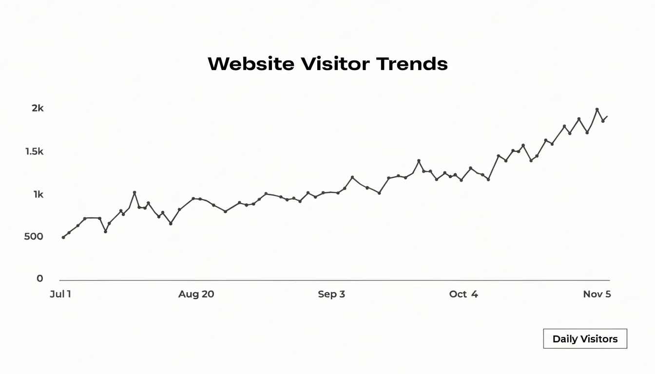
Daily user activity rarely follows a flat trajectory. Weekday and weekend patterns, promotional pushes, and referral spikes all introduce variation that can be difficult to interpret from a table of raw numbers. A line chart surfaces those fluctuations directly, allowing viewers to spot the slow days and the busy ones and to compare one week against the next. Seasonal dips become visible as recurring downward slopes at predictable points in the calendar, which helps teams anticipate quieter periods and plan content or campaigns around them.
One of the strongest advantages of the line chart is its ability to show long-term visitor growth. When the reporting window spans several months or a full year, the line smooths out short-term noise and exposes the underlying trend. A gently rising line signals steady audience expansion, while a flattening or declining line prompts closer investigation. Because the horizontal axis represents a continuous span of time, the chart also supports overlaying a second series, such as sessions or returning visitors, so daily activity and overall growth can be read together within a single view.
Bar Chart
A bar chart turns the question of where your audience lives into a ranked list you can read at a glance. Each geographic region — country, state, city, or sales territory — occupies its own category on the horizontal axis, and the length of its corresponding bar encodes a single measure such as visitor count, sessions, or conversion volume. Because the categories are discrete and unordered in the underlying data, the chart supplies the ordering itself, typically sorting bars from largest to smallest so the eye travels naturally from the biggest contributor down to the smallest. That arrangement lets you name your top-performing international markets within seconds, without scanning a table or mentally comparing columns of numbers.
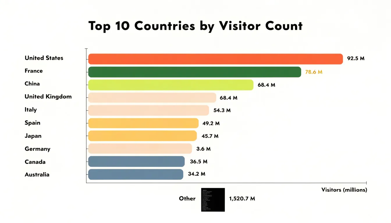
The format carries practical advantages for location data. Geographic values often have long, uneven names, and horizontal bars give those labels room to sit legibly beneath or beside each bar. The visual comparison relies on a shared baseline at zero, so proportional differences between a market with ten thousand visitors and one with two thousand read accurately as a five-to-one relationship. Viewers can also see the long tail clearly: a cluster of short bars at the bottom signals many minor markets, while a sudden drop-off indicates the point where additional localization investment is unlikely to pay off.
To keep the chart honest, limit it to roughly the top ten or fifteen regions and group the remainder into a single aggregate bar so the ranking stays readable. Keep the scale consistent across reporting periods, otherwise a growing market can appear to shrink simply because the axis stretched. Annotating the leading bars with their exact values, or layering a comparison bar for the previous period beside each current one, adds precision without cluttering the view. Handled this way, the bar chart becomes a dependable starting point for decisions about translation, currency, regional campaigns, and support coverage.
Funnel Chart
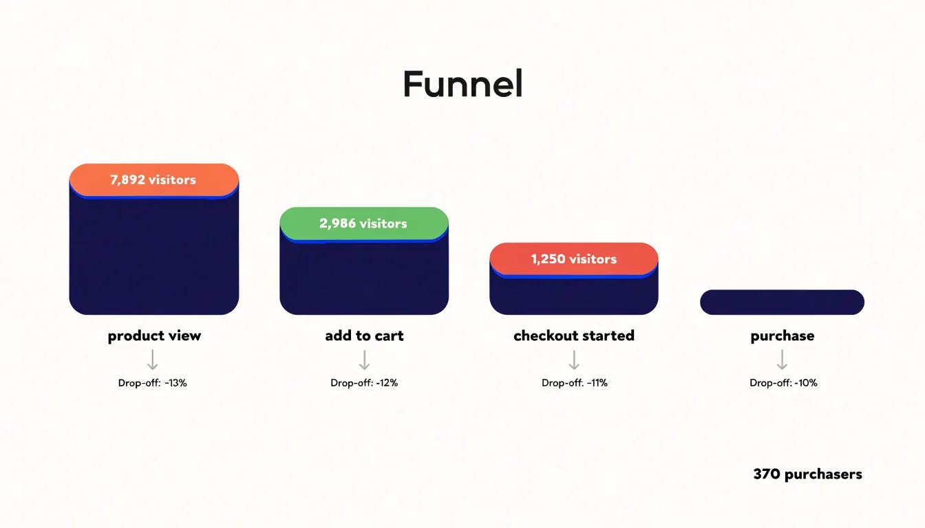
A funnel chart visualizes each stage of a multi-step conversion journey, such as a checkout process or lead-generation form, showing how many users reach each step. Starting with the total number of visitors who enter the funnel, each subsequent stage displays a progressively narrower bar, making the reduction in users immediately apparent. This visual progression highlights where the most significant drop-offs occur. For example, an e-commerce funnel might reveal that while 80% of users view a product, only 40% add it to the cart, and just 10% complete a purchase. The steepest decline between stages represents the most critical point to investigate. By pinpointing these drop-off points, you can prioritize optimization efforts, such as simplifying a form, improving page load speed, or clarifying calls to action. Funnel charts also allow for comparison across different segments or time periods, helping you assess the impact of changes. To create an effective funnel chart, ensure each stage is clearly labeled and that the data reflects a meaningful sequence. Avoid using funnel charts for non-sequential data, as the narrowing bars imply a progression that may not exist. When used correctly, funnel charts transform raw conversion numbers into actionable insights, guiding you to the steps that most need attention and ultimately improving overall conversion rates.
Pie Chart
A pie chart turns device usage into a single, immediately readable picture. Each slice represents one category of visitor, typically mobile, desktop, and tablet, and the angle of each slice corresponds to that category’s share of total sessions. Because the whole circle stands for 100 percent of traffic, viewers can grasp the rough proportions at a glance without reading a single number. When mobile visitors make up more than half the circle, that visual weight communicates a message that a table of percentages often fails to deliver with the same speed.
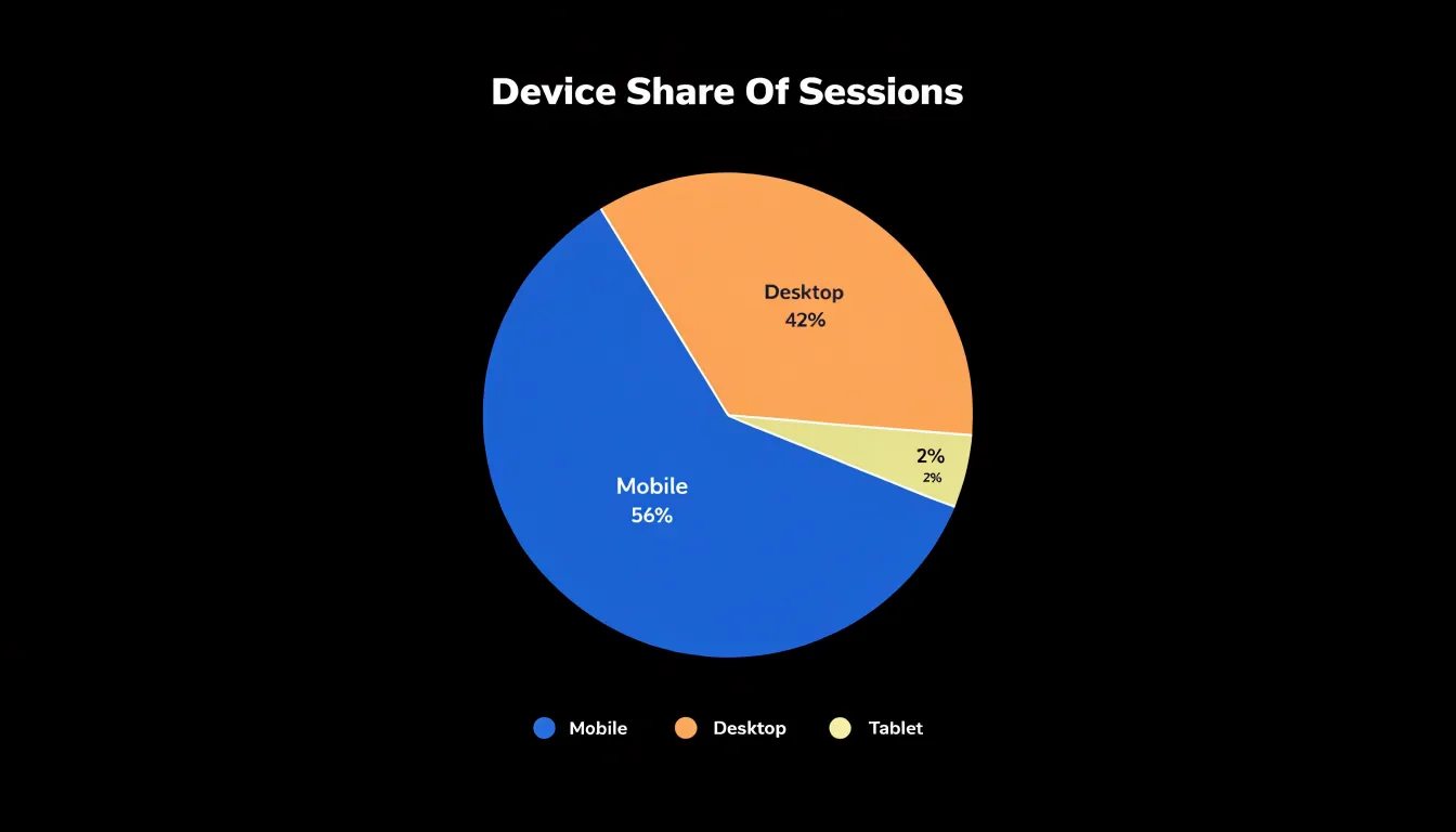
The practical value of this view lies in prioritization. Responsive web design requires trade-offs: limited development time, competing layout decisions, and finite attention to breakpoint testing. A pie chart showing device proportions gives a team a shared reference point for those decisions. If tablet traffic forms a thin sliver while desktop and mobile split the remainder, the chart offers a defensible reason to concentrate testing and optimization effort on the two dominant categories first. If the slices are closer to equal, the chart signals that every category deserves careful treatment.
For the chart to remain useful, the categories should stay few and clearly labeled. Three slices are easy to compare; eight become difficult to distinguish. Percentages placed directly on or beside each slice remove guesswork, and consistent color assignments across reporting periods make trends easier to follow when the chart is viewed repeatedly.
Pie charts also work well when the underlying data reflects a genuine whole. Device sessions naturally sum to total visits, which suits the format. Pairing the pie chart with a short caption that names the largest slice turns a decorative graphic into an actionable statement about where responsive design attention belongs.
Heat Map
Heat maps provide a visual representation of how users interact with your web pages, revealing which areas attract attention and which are overlooked. By aggregating click distributions, you can see exactly where visitors are clicking, whether on buttons, links, or non-interactive elements. This data helps identify popular elements and dead zones, allowing you to reposition key content or calls-to-action for maximum visibility. Mouse movement tracking complements click data by showing where users hover and move their cursors, which often correlates with visual attention. Even if users do not click, their mouse patterns indicate areas of interest and potential confusion. Scroll depth analysis reveals how far users scroll down a page, highlighting where they lose engagement. If a significant portion of visitors drop off before reaching a certain point, you can adjust content length or move important information higher. Combining these three metrics offers a comprehensive view of on-page engagement. For instance, you might discover that a call-to-action button receives many clicks but is placed below the average scroll depth, meaning most users never see it. Armed with this insight, you can relocate the button to a more visible area. Heat maps also help optimize user experience by identifying confusing layouts or elements that attract clicks but lead nowhere, such as non-clickable images that look like buttons. By continuously monitoring heat map data, you can iterate on design changes and measure their impact, ensuring that your website aligns with user behavior and business goals. Ultimately, heat maps transform raw interaction data into actionable insights for improving layout, content placement, and conversion rates.
Stacked Bar Chart
A stacked bar chart excels at showing how total visitor volume breaks down by acquisition channel over time. Each bar represents a time period—such as a day, week, or month—and its height reflects the total number of visitors. The bar is then divided into segments, each corresponding to a traffic source like organic search, paid search, social media, referral, or direct. This visual layout makes it easy to compare total traffic across periods while simultaneously seeing the contribution of each channel. For example, you might notice that while overall traffic is growing, the growth is driven entirely by paid search, while organic search remains flat. Such insights are critical for evaluating the composition of your marketing channel mix. By stacking the segments, you can quickly assess which channels are gaining or losing share over time. The chart also helps identify seasonal patterns or the impact of campaign launches on specific channels. When designing a stacked bar chart for analytics, ensure that the number of segments is manageable—typically five to seven—to avoid clutter. Use distinct colors and a legend for clarity, and consider adding percentage labels if the relative proportions are more important than absolute numbers. Keep the time axis consistent to facilitate trend analysis. Overall, the stacked bar chart provides a balanced view of both total volume and channel composition, making it an indispensable tool for marketing analysts who need to communicate the effectiveness of their acquisition strategies.
Heatmap Grid
A heatmap grid turns a full week of traffic data into a single visual field, with days of the week running along one axis and hours of the day along the other. Each cell represents the intersection of a specific day and hour, and its color intensity reflects how much activity occurred during that window. Darker or warmer cells mark the busiest periods, while lighter cells reveal the quiet stretches. This arrangement lets you absorb an entire week’s rhythm at a glance, something a table of raw numbers or a line chart with dozens of overlapping series cannot deliver as quickly.
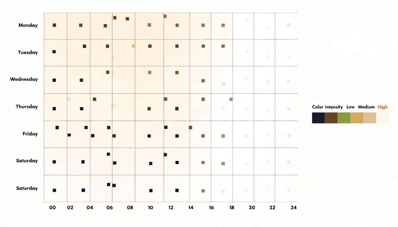
Reading the grid begins with locating the clusters of intense color. A block of dark cells spanning weekday mornings, for example, tells you when a substantial share of your audience is already online and engaged. Those windows are prime candidates for publishing new content, since a fresh post will meet the largest available audience right away. Equally useful are the pale zones: weekend afternoons or late-night hours where traffic thins out. Scheduling a major launch there means fewer eyes on the announcement during its first critical hours.
The same logic applies to campaigns. If you plan an email send, a social push, or a paid promotion, the grid shows which hours historically carry the most visitors, so the campaign lands when people are present to see it. Recurring patterns across several weeks add confidence, and comparing one grid against another, such as this month versus last, reveals shifts in audience behavior over time.
Practical use of the heatmap grid depends on clean hourly data grouped by day. Most analytics platforms can generate this view directly, and a consistent color scale keeps busy and quiet periods easy to distinguish at a glance.
Sankey Diagram
A Sankey diagram renders flow as a set of connected bands whose width is proportional to the volume of traffic moving through each stage, which makes it a natural fit for mapping how visitors travel through a website. The diagram begins with an entry point, typically segmented by traffic source, landing page, or device type, and then branches outward across each subsequent interaction. Each band thickens or narrows as users move from one page or event to the next, so the relative popularity of every step is visible at a glance without requiring a table of numbers.
The real value of this visualization appears when navigation involves three, four, or more steps. Simple funnel charts capture linear drop-off, yet most browsing behavior is anything but linear. Visitors hop between product pages, circle back to the homepage, open a help article, and return to a category listing. A Sankey diagram can hold all of those branches in a single view, showing where paths diverge and where they converge again. Common user journeys become obvious because the widest ribbons trace the routes that most people follow, from landing page through mid-funnel pages to checkout, signup, or another conversion event.
The unexpected patterns often prove just as useful. A surprisingly thick band heading from a pricing page to a support article may reveal unanswered questions about plans. A narrow but persistent stream looping between two pages might point to confusing navigation or a broken link. Segments that terminate abruptly can highlight friction points where users abandon the journey.
Because the diagram depends on clean, sequential event data, it works best when pageviews or events are logged in order with consistent identifiers. Used thoughtfully, a Sankey diagram turns raw navigation logs into a map of user intent, guiding layout changes, content placement, and conversion optimization.
Tree Map
A tree map organizes page popularity as a set of nested rectangles, where the full canvas represents total site traffic and each rectangle stands for a page, section, or content group. The size of every rectangle is proportional to its share of visits, so a reader can scan the chart and immediately see which content sections dominate the site’s audience attention. Unlike a ranked table of URLs, the tree map keeps hierarchical structure visible: a parent rectangle for a blog category contains smaller rectangles for its individual articles, letting analysts see whether a category’s traffic comes from one breakout page or from steady contributions across many posts. Color adds a second variable, such as bounce rate, conversion rate, or average session duration, so a large rectangle tinted in a warning hue signals a high-traffic section that fails to engage its visitors.
This layout makes underutilized site assets easy to spot. Small rectangles tucked into corners of the canvas reveal pages that receive little traffic relative to their importance in the site structure, giving content teams a clear shortlist for optimization, internal linking, or retirement. Comparing two tree maps side by side across different time periods shows how page popularity shifts after a redesign or campaign, since rectangle proportions change visibly as traffic moves between sections.
The chart works best when page names stay short and the hierarchy stays shallow, typically two or three levels deep, because deeper nesting shrinks labels until they become unreadable. Grouping long-tail URLs into buckets such as “archived posts” or “miscellaneous pages” prevents hundreds of tiny slivers from cluttering the canvas. With that preparation, a tree map turns raw pageview data into a quick visual audit of which content sections earn their place on the site and which ones deserve renewed attention.
Cohort Chart
A cohort chart groups users by the period in which they first signed up, then tracks how each group behaves over subsequent weeks or months. Rather than viewing all users as a single blended average, the chart separates signup groups into distinct rows, with each row showing the percentage of that group still active at each interval after signup. This structure reveals whether retention is improving or deteriorating across successive cohorts, which a single aggregate retention number tends to obscure.
Tracking these signup groups across weekly or monthly intervals provides a clear picture of product-market fit. When newer cohorts retain better than older ones, the product is likely resonating more strongly with each incoming wave of users. When retention curves flatten early and hold steady, that plateau indicates a core group finding lasting value. When curves drop steeply and continue declining, the product may be attracting users whose needs it does not fully meet, and the chart makes that pattern visible before it becomes a larger revenue problem.
Cohort charts also support churn rate calculation with precision. By comparing the active percentage at one interval against the previous interval within the same cohort, you can derive period-over-period churn for that specific group. Aggregating across cohorts produces a more reliable churn estimate than a simple snapshot of total active users, since it accounts for the age of each user base. These calculations feed directly into forecasts for lifetime value, support staffing, and acquisition targets.
The chart works best when cohorts are defined by a meaningful shared start event, such as first signup, first purchase, or first meaningful action. Weekly intervals suit fast-moving products with short activation cycles, while monthly intervals suit products with longer consideration periods. Pairing the cohort view with segmentation by acquisition channel or plan type sharpens the analysis further, showing which entry paths produce the strongest long-term retention.
Area Chart
An area chart is well suited to tracking campaign growth over time, particularly when the goal is to understand how individual marketing channels contribute to an overall cumulative volume. The chart lays a series of filled areas on top of one another, with the vertical position of each band representing a single channel’s contribution and the combined height representing the total. This stacking approach lets a viewer read two stories at once: the overall trajectory of the campaign and the relative weight of each channel driving that trajectory. When a campaign launches across search, social, email, and display, the area chart shows at a glance which channel is expanding fastest and whether the total reach is climbing steadily, plateauing, or tapering off. Because the filled regions are continuous across the horizontal axis, the chart communicates flow and momentum in a way that isolated data points or a plain table cannot. Viewers can trace the shape of growth week by week and see where a channel’s band widens or narrows, which often corresponds to a budget shift, a creative refresh, or a seasonal effect. Color coding keeps the channels distinct, while a shared legend and consistent axis scale preserve clarity. For reporting to stakeholders, the area chart offers a compact summary of reach accumulation, making it easy to compare the total volume achieved in one period against another. It also supports annotation, so key moments such as a campaign launch or a promotional push can be marked directly on the chart. This combination of total trend and channel-level detail makes the area chart a practical choice for demonstrating growth and attributing it across the channels that produced it.
Scatter Plot
Scatter plots offer a clear way to examine the relationship between two numeric variables, and one practical use is reviewing site speed. By plotting each page’s load time on one axis against a metric such as bounce rate on the other, you create a visual field of individual data points where each dot represents a single page. This arrangement lets you spot patterns and outliers at a glance rather than sorting through rows of a table. Pages clustered in the upper right corner, with long load times and high bounce rates, stand out immediately as candidates for optimization. Conversely, pages near the lower left combine fast loading with lower bounce rates, showing where performance is already strong. The spread of points also reveals whether a relationship exists between speed and engagement across your site. A general upward trend suggests that slower pages tend to lose visitors, while a scattered cloud with no clear direction may indicate that other factors, such as content quality or traffic source, play a larger role. Color-coding points by page category, device type, or traffic channel adds another layer of insight, helping you see whether the pattern holds across segments. With interactive tooltips, hovering over a point can display the page URL, exact load time, and bounce rate, making follow-up investigation straightforward. The scatter plot works best when paired with a clear reference line or threshold marking an acceptable load time, giving viewers a benchmark against which to judge each point. Used this way, the chart turns raw speed and engagement data into an actionable map of where to focus technical improvements.
Horizontal Bar Chart
A horizontal bar chart provides a clear view of form completion by displaying field-by-field engagement rates. Each bar represents a form field, and its length corresponds to the percentage of users who successfully complete that field. This layout makes it easy to compare engagement across fields and identify where users drop off. By ordering fields from top to bottom in the same sequence they appear on the form, the chart mirrors the user’s journey, allowing you to spot the exact input where friction occurs. For instance, if a field asking for a phone number shows a significantly shorter bar than preceding fields, it signals that users are abandoning the form at that point. The horizontal orientation is particularly effective for forms with many fields or long labels, as it accommodates text without truncation and keeps the chart readable. You can further enhance the chart by color-coding bars to indicate completion thresholds, such as green for high engagement and red for low, drawing immediate attention to problematic areas. Additionally, adding data labels with exact percentages provides precise insights. When analyzing form abandonment, the horizontal bar chart helps pinpoint specific inputs that cause users to hesitate or leave. This could be due to unclear instructions, privacy concerns, or technical issues like validation errors. By addressing these friction points, you can streamline the form and improve overall completion rates. To maximize the chart’s usefulness, segment the data by user demographics or traffic sources to uncover patterns—for example, mobile users might struggle with certain fields more than desktop users. Regularly updating the chart as you make changes allows you to track the impact of your optimizations. In summary, the horizontal bar chart is an indispensable tool for diagnosing form engagement and reducing abandonment by making field-level performance immediately visible.
Combo Chart
A combo chart overlays two different chart types on a single set of axes, most commonly pairing bars with a line. This structure suits whole-site dashboards particularly well, where the goal is to show the health of the site at a glance and let viewers connect two metrics that tell a fuller story together. Total sessions, for example, might be plotted as bars along the bottom of the chart, giving a sense of volume month by month, while conversion rate runs as a line across the same period. Because the two metrics carry very different scales, the bars can use a left axis sized for raw counts and the line a right axis sized for percentages, so neither series gets flattened or exaggerated by the other.
The value of this arrangement appears when the two metrics move in different directions or at different rhythms. A month where sessions climb sharply while the conversion line dips suggests traffic quality has shifted, perhaps from a new campaign bringing in less qualified visitors. A flat bar profile with a rising line points to better on-site performance rather than more visitors. On a single dashboard these patterns become visible without requiring the reader to flip between charts or hold numbers in memory. The bars set the context of scale, and the line adds the efficiency story on top of it.
When building these dashboards, keep the design restrained. Limit the chart to two series, use distinct colors that match the legend, and label both axes clearly so the dual scale is never ambiguous. Keep bar widths consistent and avoid stacking multiple bars behind the line, which muddies the reading of volume. With those conventions in place, a combo chart becomes a compact summary that grounds a website analytics dashboard in both traffic and outcomes.
Frequently Asked Questions
What chart is best for tracking daily website traffic?
A line chart is a natural fit for daily traffic tracking because it plots each day’s visitor count along a continuous time axis and connects the points to show direction and momentum. It also helps reveal fluctuations and long-term visitor growth.
How many regions should I include in a bar chart of website location data?
Limit the bar chart to roughly the top ten or fifteen regions and group the remainder into a single aggregate bar so the ranking stays readable. Keep the scale consistent across reporting periods so a growing market does not appear to shrink because the axis stretched.
When should I use a funnel chart in website analytics?
Use a funnel chart to visualize each stage of a multi-step conversion journey, such as a checkout process or lead-generation form, and show where users drop off. Avoid using funnel charts for non-sequential data because the narrowing bars imply a progression that may not exist.
What can a heat map show about how users interact with a web page?
Heat maps aggregate click distributions to show where visitors click, and they can also include mouse movement and scroll depth data. This helps identify popular elements, dead zones, and places where users lose engagement, such as a call-to-action below the average scroll depth.
How do I read a heatmap grid for website traffic?
A heatmap grid shows days of the week along one axis and hours of the day along the other, with cell color intensity reflecting activity in each window. Darker or warmer cells mark busiest periods, while lighter cells show quiet stretches, helping you choose when to publish content or run campaigns.
How does a cohort chart help analyze user retention?
A cohort chart groups users by the period they first signed up and tracks the percentage still active at later intervals. It shows whether retention is improving or deteriorating across cohorts and supports more precise churn-rate calculation.
Tony Astor
Tony writes about data visualization and the tools people use to build charts and dashboards. More about Data Illustrator