Best Charts for Scientific Papers and Research
 By Tony Astor ·

Best Charts for Scientific Papers and Research
Use bar graphs for discrete comparisons, line charts for time-series trends, scatter plots for variable relationships, histograms for distributions, box plots for five-number summaries, heat maps for dense matrices, and forest plots for meta-analysis effect sizes. Match chart type to data structure, label axes with units, include error bars, avoid truncated axes, and follow journal resolution and color-space guidelines.
Table of Contents
Bar Graphs
Bar graphs excel at comparing discrete categories, such as experimental groups, survey responses, or species counts. Begin by ordering categories logically—either by magnitude or by a meaningful sequence like time or treatment level—to guide the reader’s eye. Use consistent bar widths and spacing to avoid visual distortion.
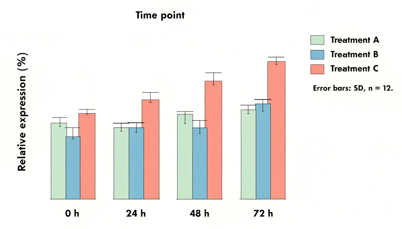
When displaying summary statistics, always include error bars to convey variability or uncertainty. Specify in the caption whether error bars represent standard deviation, standard error, or confidence intervals, and state the sample size.
For comparisons across multiple conditions, grouped bar graphs can work, but limit the number of groups to prevent visual clutter. If your graph has more than three or four groups, consider a different chart type or split the data into multiple panels. Avoid overcrowding by not stacking too many categories; stacked bars are useful for showing part-to-whole relationships but can obscure individual comparisons. Instead, use a single bar per category when the focus is on direct comparison.
Keep colors distinct and accessible, and label axes clearly with units. Finally, avoid 3D effects or excessive decoration, which can distort perception.
Line Charts
Line charts are a natural choice when a study unfolds across time. They connect individual observations into a continuous path, letting readers perceive direction, pace, and inflection points. When plotting longitudinal data, confirm that your measurements share a consistent time base, such as weeks since enrollment or months since treatment initiation, so that distance along the horizontal axis reflects real elapsed time. Place the continuous variable on the vertical axis and keep scaling consistent across panels to avoid distorting perceived rates of change. If several groups are compared, assign each a distinct line style or color and repeat the legend or annotate the lines directly where space allows.
Clear time-series changes come from reducing visual noise. Light gridlines, restrained colors, and a single plotting layer help the trend command attention. Where measurements are irregular, markers can indicate actual observation points while the connecting line shows continuity. Confidence bands or error bars may be added sparingly where they support interpretation rather than clutter. Consider annotating key events, such as a change in protocol or an intervention, with a vertical reference line and a short label.
Interval markers deserve deliberate thought. Too many tick marks crowd the axis and obscure labels, while too few can hide meaningful variation. Choose intervals that match the rhythm of data collection, such as monthly ticks for monthly measurements, and label them in a readable format. If the time span is long, consider summarizing with quarterly or annual ticks and stating the granularity in the caption. Keep tick spacing uniform unless a deliberate broken axis is justified and clearly flagged.
Scatter Plots
Scatter plots place one continuous variable on the horizontal axis and another on the vertical axis, with each point representing a single observation. The resulting cloud of points reveals the relationship between the two variables, showing whether values rise together, move in opposite directions, or show no discernible pattern. Before running formal statistical tests, a scatter plot allows researchers to see the shape of the association, whether it is linear or curved, how tightly the points cluster around an implied trend, and whether the spread of one variable changes across the range of the other. Outliers and unusual observations are also easy to identify, since they sit apart from the main body of data and can prompt a closer look before they distort an analysis.
Adding a regression line turns the scatter plot into a compact summary of the association. A fitted line shows the direction and steepness of the relationship, and including a confidence band around it communicates the precision of the estimate across the observed range. When several groups appear in the same dataset, plotting them with distinct markers or colors and fitting separate lines for each group makes it possible to compare slopes and intercepts directly, helping to judge whether an apparent trend holds across conditions or is driven by a single subgroup.
Scatter plots also support the identification of statistical clusters. Dense regions of points, gaps between them, and separate islands of observations can reveal latent structure in the data, such as distinct populations or measurement regimes. Annotating clusters with labels, using transparency to handle overplotting, and adding marginal histograms or density contours all help readers see where the mass of the data lies.
Histograms
Histograms visualize the distribution of continuous data by grouping observations into logical bins and displaying the frequency within each interval, revealing the shape of the underlying probability distribution. The choice of bin width is critical: too few bins oversimplify the data and obscure important features, while too many bins introduce noise and make the distribution hard to discern. A common rule of thumb is to use the square root of the number of data points as a starting point for the number of bins, but researchers should experiment with different bin widths to find a clear and informative representation.
Ensure that bins are of equal width and cover the entire range of the data without overlap. The y-axis can represent either the count of observations in each bin or the density (count divided by bin width and total count), which allows for comparison across datasets with different sample sizes. For scientific papers, it is often beneficial to overlay a kernel density estimate or a fitted theoretical distribution to provide a smoother representation of the data’s shape and to facilitate interpretation.
Histograms are particularly useful for identifying skewness, multimodality, and outliers. However, they can be sensitive to the starting point of the bins, so it is good practice to report the binning strategy in the figure legend. Additionally, for small datasets, histograms may not be the best choice; dot plots or stem-and-leaf plots can be more appropriate.
Box Plots
Box plots summarize the distribution of a dataset using the five-number summary: the minimum, first quartile, median, third quartile, and maximum. The median marks the central tendency of the sample, giving readers an immediate sense of the typical value without being distorted by unusually high or low observations. The first and third quartiles define the interquartile range, which contains the middle fifty percent of the data and provides a robust measure of variability that resists the influence of extreme values.
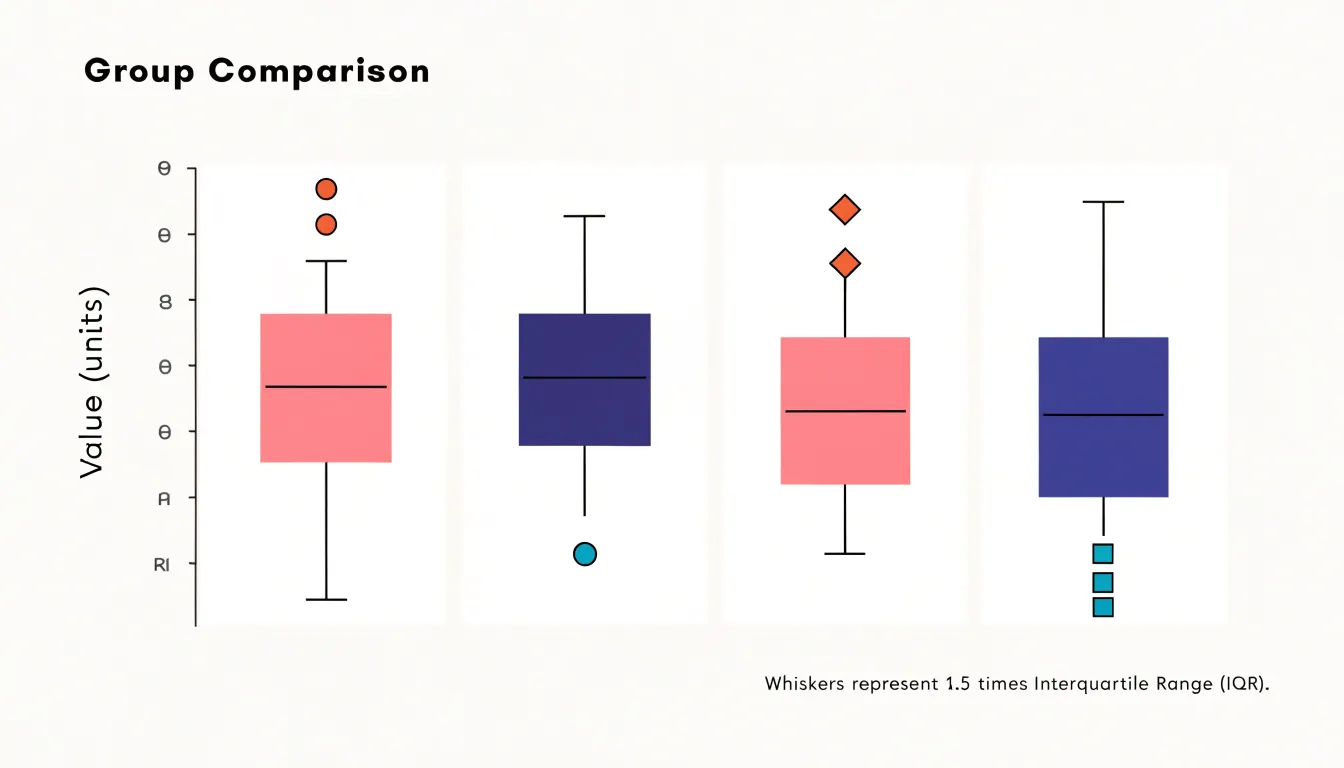
One of the greatest strengths of the box plot is how it handles outliers. Observations that fall far below the first quartile or far above the third quartile can be plotted individually as distinct points, drawing attention to statistical anomalies, experimental errors, or genuinely rare phenomena that might otherwise be buried in a table of raw numbers. Because the central box and whiskers remain unaffected by these extreme points, the reader can simultaneously see the core structure of the data and the presence of exceptional values.
Box plots also excel at facilitating comparison across groups. When several boxes are placed side by side, differences in medians, spreads, and outlier patterns become immediately visible, allowing researchers to assess variation between experimental conditions, populations, or treatments in journal articles where space is limited.
Heat Maps
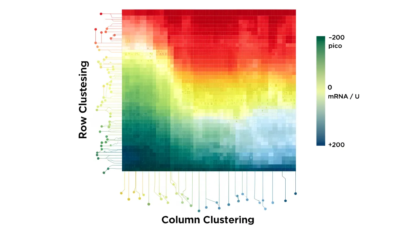
Heat maps translate numerical values into color, letting readers scan a dense grid and spot clusters, outliers, and gradients. Each cell in the matrix receives a shade drawn from a defined color gradient, so the eye can compare hundreds or thousands of data points simultaneously without tracing individual numbers.
In gene expression studies, for example, rows typically represent genes and columns represent experimental conditions or time points. Standardizing values across rows before mapping them to color ensures that upregulation and downregulation stand out against each gene’s own baseline, revealing co-expressed gene modules and condition-specific signatures. The same principle applies to correlation matrices, where each cell encodes the strength and direction of a relationship between two variables; diverging palettes with a neutral midpoint at zero make positive and negative correlations immediately distinguishable.
Sequential palettes suit data that run from low to high, while diverging palettes fit values centered on a meaningful midpoint. Perceptually uniform colormaps avoid the false boundaries and misleading brightness jumps that older rainbow schemes introduce, and they remain legible for readers with color vision deficiencies.
Dendrograms added along the rows and columns, producing clustered heat maps, group similar profiles together and expose block structures that raw tables obscure. Include a labeled color bar with units and state the normalization method in the caption to help readers interpret the figure correctly. When the underlying matrix is large, researchers often pair the heat map with a smaller inset or supplementary table so specific values remain accessible.
Pie Charts
Pie charts serve a narrow purpose in scientific publication: displaying simple part-to-whole relationships where a small number of categories together form a meaningful total. When a sample divides into a handful of distinct groups, a pie chart can communicate the relative sizes of those groups, giving readers an immediate sense of which categories dominate and which are marginal. This works best when the proportions are clearly different from one another, so that visual differences correspond to real differences in magnitude rather than forcing readers to compare near-identical wedges.
Strict limits on slice counts must be maintained because the human visual system is poor at estimating angles and arc lengths. Reviewers and readers cannot reliably judge whether one wedge is 18 percent or 22 percent of the whole, and the difficulty increases as slices become thinner. Beyond roughly five or six categories, the chart collapses into a cluster of slivers that convey little beyond the presence of many small groups. In these situations, the part-to-whole message is better served by a stacked bar chart or a simple table, both of which support accurate comparison.
Journals often print figures at reduced size or in greyscale, so wedges that differ only subtly in hue may become indistinguishable. Labeling every slice with a percentage and category name, and ordering slices from largest to smallest, helps preserve readability. Small categories can be grouped into an explicit “other” category when their individual identities matter less than the overall structure of the data.
Authors should also consider whether the total is genuinely meaningful. Pie charts imply that the parts exhaust the whole, so they suit composition data such as the breakdown of a sample by treatment arm or the distribution of responses across mutually exclusive options.
Bubble Charts
Bubble charts extend the two-dimensional scatter plot by scaling the area of each marker in proportion to a third quantitative metric. This allows a single visual to communicate three measurements simultaneously without resorting to multiple panels or complex overlays. The technique is especially useful in epidemiology, economics, environmental science, and engineering, where datasets often include a natural third variable like population size, sample count, funding level, or concentration.
Researchers should scale marker area rather than diameter, because human perception interprets the overall area of a shape more accurately than its width. Clear legends that map marker sizes to specific values help readers decode the third variable, and consistent color or outline styling can distinguish categories or highlight important subsets.
Because large bubbles can overlap and obscure smaller ones, thoughtful ordering of plotting layers and moderate transparency are helpful practices. Labeling only the most significant points keeps the visual uncluttered while preserving interpretability. When done well, bubble charts encourage readers to notice patterns that a simple scatter plot would miss, such as clusters of large values in a particular region of the plane or an inverse relationship between the third metric and the two axis variables.
Area Charts
Area charts show cumulative totals over time, with each series stacked on top of the previous one so the total height of the chart reflects the combined volume at any given point. This makes them well suited to research contexts where the question is how several contributing components add up across a study period, such as cumulative sample counts, aggregated energy use, or the buildup of measured outcomes across experimental phases. The filled areas draw attention to the overall magnitude of change, and the layered structure lets readers see both the total and the share contributed by each category at once.
Baseline consistency is essential. Every series should begin from the same zero point, and the y-axis should remain linear across the full plotting area so that the height of each band corresponds directly to its value. Inconsistent baselines or truncated axes distort the relative size of the stacked segments and can suggest trends that the underlying data do not support. Readers should also be able to trace each series back to a clearly labelled zero reference, particularly when the chart appears at small print sizes.
Stacked areas can obscure one another when values fluctuate sharply or when a smaller series sits behind a larger one. Ordering series from largest to smallest at the base of the stack, limiting the number of categories, and using distinct fills with consistent colour encoding all help keep every band legible. Where overlap cannot be avoided, data labels and a well-placed legend reduce ambiguity.
Violin Plots
Violin plots pair a kernel density estimation with the metrics of a box plot, giving a single figure that carries both distributional shape and summary statistics. The mirrored density curve on either side of the central axis smooths the observed data into a continuous profile of where values cluster. The width of that curve at any point reflects the local density of observations, so thicker sections indicate ranges where more data points fall and narrower sections mark sparse regions. Superimposed on this shape is a compact box plot, typically showing the median, the interquartile range, and often whiskers or markers for individual points.
This combination exposes features that simpler summaries can obscure. A histogram or a plain box plot can collapse a dataset into a single lump, whereas the violin’s contour can reveal multi-modal distributions, where two or more distinct peaks indicate subpopulations hidden within a pooled sample. Researchers comparing treatment groups, experimental conditions, or demographic cohorts can observe whether differences arise from shifts in central tendency, changes in spread, or the emergence of secondary clusters. The overlaid box metrics anchor the smoothed density to concrete numbers, so readers can judge the median and quartiles alongside the overall silhouette.
Because kernel density estimation introduces smoothing and the appearance of the curve depends on bandwidth selection, authors typically note the method used and present the raw points when sample sizes are small. Violin plots work best when placed side by side across categories, using consistent axes and color to support direct comparison.
Forest Plots
Forest plots summarize results from multiple studies in a meta-analysis. They display each study’s effect size as a point estimate, typically represented by a square whose size reflects the study’s weight or precision. Horizontal lines extending from each square denote the confidence interval, providing a range within which the true effect is likely to lie. Wider intervals indicate greater variability or smaller sample sizes.
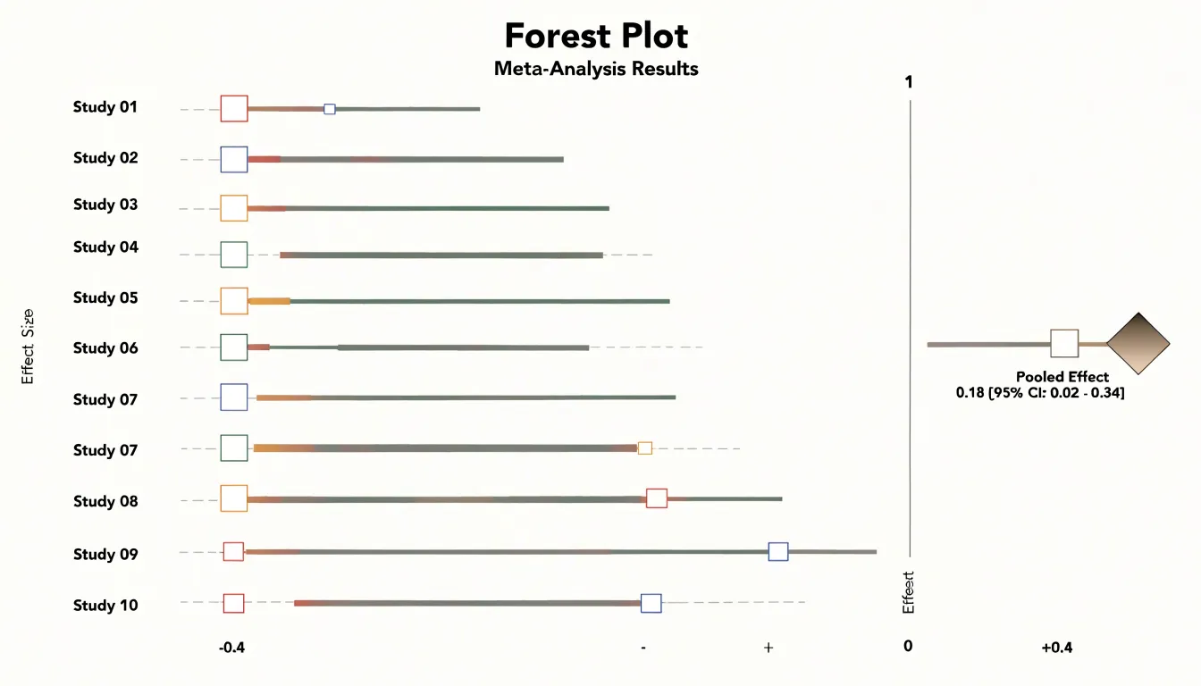
A vertical line, often placed at the null effect value (e.g., an odds ratio of 1 or a mean difference of 0), serves as a reference point for interpreting whether individual studies show a positive, negative, or null effect. When confidence intervals cross this line, the result is generally considered not statistically significant at the chosen level.
The overall pooled estimate is typically represented by a diamond at the bottom of the plot. The center of the diamond indicates the combined effect size, while its width spans the confidence interval for the pooled result, synthesizing evidence across studies.
Forest plots also facilitate the assessment of heterogeneity—variation in effect sizes beyond what would be expected by chance. By visually inspecting the spread of study estimates and their overlap with the pooled estimate, readers can gauge consistency. Labels often include numerical data such as effect sizes, confidence intervals, and weights, allowing for detailed verification in evidence synthesis and systematic reviews.
Flowcharts
Flowcharts translate a sequence of actions into a visual grammar that makes a study’s methodology auditable: each box represents a discrete step, each arrow fixes the order of operations, and each labeled branch records a condition that determines what happens next.
- Laboratory protocols: Step-by-step diagrams separate preparation, intervention, and measurement phases, annotate timing and quantities where they matter, and keep symbols consistent so that readers can trace any pathway from start to finish.
- Decision trees: These foreground the logic of branching choices, such as whether a sample qualifies for analysis, which instrument setting applies under a given condition, or how an ambiguous result is resolved. Exposing the rules governing each fork reduces the chance that a reader misinterprets a conditional step buried in a paragraph.
- CONSORT-style participant flow diagrams: These apply the format to study enrollment and retention, showing the number of individuals assessed for eligibility, excluded and why, randomized to each arm, and followed through to analysis. They make attrition visible and allow reviewers to check that reported denominators match the actual population studied.
Across all three applications, clarity depends on a consistent direction of flow, concise labels, explicit counts at each stage, and grouping that mirrors the study design itself.
Chart Integrity
Readers rely on visual representations to understand data they may never examine in its raw form. A chart that distorts the underlying numbers, even unintentionally, undermines the credibility of the research and can lead to unsupported conclusions.
The most common source of distortion is the truncated axis, where the vertical scale begins at a value other than zero. While truncation can be legitimate when the data range is narrow and the zero point is irrelevant, it exaggerates differences between values and makes small variations appear dramatic. Authors should state clearly when an axis is truncated and justify the choice in the caption.
Equally problematic is erratic scaling, in which intervals between tick marks change without notice or the axis jumps between units. Inconsistent spacing compresses some portions of the data and expands others, producing a visual rhythm that misrepresents the actual relationships. Readers absorb the shape of a curve or the height of a bar before they read the labels, so irregular scaling exploits that first impression.
Manipulated visual proportions present a subtler challenge. Changing the aspect ratio of a plot can flatten or steepen trends, and using area or volume to encode a single variable can magnify differences far beyond their true magnitude. Pie charts with exaggerated segments and three-dimensional effects that obscure the true heights of bars fall into the same category. Maintaining ethical visual standards requires consistent axes, honest proportions, clear labeling, and transparent disclosure of any necessary adjustments.
Design Software
The choice of design software shapes both the workflow and the final visual quality of scientific figures.
- R (ggplot2): Offers a grammar-of-graphics approach to produce reproducible plots directly from raw data, suiting researchers who manage large datasets or need to regenerate figures consistently across revisions.
- Python (Matplotlib, Seaborn, Plotly): Provides programmatic control and integrates naturally into analysis pipelines.
- GraphPad Prism: Combines statistical analysis with a point-and-click interface that many experimental biologists find efficient for standard chart types, dose-response curves, and survival plots.
- Adobe Illustrator: Functions as a finishing tool for post-processing exported figures, adjusting typography, aligning panels, and preparing artwork that meets journal specifications.
Programmatic tools reward users who need precise control over every aesthetic element and value scripted reproducibility, though they demand familiarity with code. Prism reduces the learning curve for common analyses but can feel limiting when a figure calls for unusual layouts or fine-grained styling. Illustrator excels at manual refinement but is poorly suited to generating plots from data, so it typically complements rather than replaces analytical software.
Journals often specify minimum resolution, file formats such as TIFF, EPS, or PDF, embedded fonts, color modes, and accessible color palettes. Some publishers also request vector output for line art, which narrows the viable export pathways. Matching software to these requirements early prevents time-consuming rework when a manuscript nears submission.
Style Guides
Physical and digital production imposes constraints that a draft manuscript never encounters, and the responsibility for meeting a publisher’s specifications rests with the author.
Resolution requirements are usually the first hurdle. Most publishers state a minimum of 300 dots per inch (dpi) for raster images such as photographs, gels, and micrographs, while line art and combination figures may demand 600 to 1200 dpi so that thin strokes and small labels remain legible. Submitting a figure at screen resolution, often around 72 to 96 dpi, produces visible pixelation once the journal scales it to column width.
Publishers also specify acceptable typefaces, minimum font sizes after scaling, and consistent label formatting across all figures, with some requiring that lettering match the journal’s own design conventions. Text that reads clearly at full page width may become unreadable when the figure is reduced to a single column, so labels should be set with the final printed dimensions in mind.
Color space rules complete the checklist. Print workflows rely on CMYK, a subtractive model built from cyan, magenta, yellow, and black inks, while screens and most microscopy software output RGB, an additive model. Bright saturated RGB hues can shift or dull when converted, so authors preparing for print journals should convert color figures to CMYK and inspect the result rather than trust an automatic conversion. Online-only publications often prefer RGB or sRGB, and some journals ask for both versions. Reviewing the target journal’s author guidelines before finalizing figures saves revision cycles and prevents last-minute reformatting.
Frequently Asked Questions
How do I decide between a bar graph and a line chart for my research data?
Bar graphs are used to compare discrete categories, such as experimental groups, survey responses, or species counts, while line charts are a natural choice when a study unfolds across time. Line charts connect individual observations into a continuous path so readers can perceive direction, pace, and inflection points.
What should I state in the caption about error bars?
When displaying summary statistics, include error bars to convey variability or uncertainty. In the caption, specify whether the error bars represent standard deviation, standard error, or confidence intervals, and state the sample size.
How many bins should I use for a histogram?
A common rule of thumb is to use the square root of the number of data points as a starting point for the number of bins, but researchers should experiment with different bin widths to find a clear and informative representation. The article also says bins should be equal width and cover the entire data range without overlap.
How many slices should a pie chart have?
Pie charts should be limited to a small number of categories, and beyond roughly five or six categories the chart collapses into slivers that convey little. For more categories, a stacked bar chart or simple table better supports accurate comparison.
What is a violin plot used for?
A violin plot pairs a kernel density estimate with box plot metrics, showing distributional shape and summary statistics in one figure. It can reveal multi-modal distributions that simpler summaries might obscure, and it works best when placed side by side across categories with consistent axes and color.
Can I truncate the y-axis in a scientific chart?
Truncation can be legitimate when the data range is narrow and the zero point is irrelevant, but it exaggerates differences between values. Authors should state clearly when an axis is truncated and justify the choice in the caption.
Tony Astor
Tony writes about data visualization and the tools people use to build charts and dashboards. More about Data Illustrator