Best Charts for Sales Data and Revenue Trends
 By Tony Astor ·

Best Charts for Sales Data and Revenue Trends
The best chart for sales data depends on the question: line graphs track revenue trends and seasonality over time, bar charts compare performance across categories, stacked bars show totals and components together, and waterfall charts bridge gross revenue to net profit. Pie charts suit static composition, funnels expose pipeline drop-off, and scatter plots reveal price-volume relationships.
Table of Contents
Line Graphs
Line graphs serve as the default choice for tracking revenue trends because they treat time as a continuous dimension, connecting each data point to its neighbors to reveal the shape of change rather than isolated snapshots. Plotting monthly revenue along a horizontal time axis turns discrete numbers into a visible trajectory. A sales manager can immediately read whether revenue is climbing, plateauing, or declining, while the line’s slope communicates the pace of movement. This makes line graphs especially effective for annual comparisons: plotting multiple years as separate lines on the same axes lets viewers compare growth rates and spot years that broke from historical patterns.
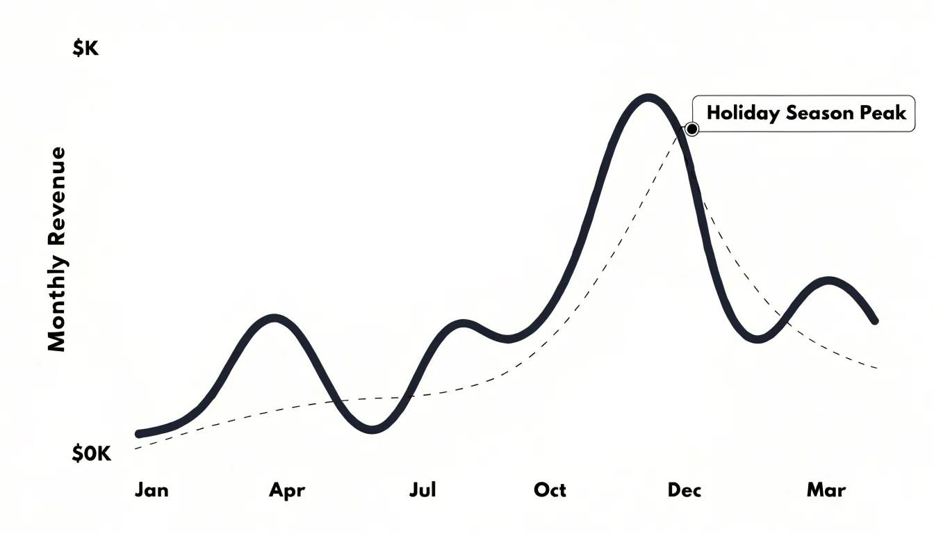
The format also exposes seasonality. Because revenue typically swells during holiday quarters, dips in slower months, and rebounds predictably, a line graph renders these rhythms as a repeating wave rather than scattered points. Analysts can overlay a trendline or moving average to separate the seasonal signal from the underlying growth trajectory, clarifying whether an apparent gain reflects genuine expansion or a routine seasonal upswing. Color-coded segments, annotated peaks, and shaded regions can highlight periods of interest without obscuring the overall shape.
Line graphs scale well across time horizons. Daily or weekly plots capture short-term volatility, while monthly and quarterly aggregations smooth noise to reveal strategic direction. Because the visual encoding relies on position along a common axis, viewers can compare values precisely and evaluate what happens between recorded intervals.
Bar Charts
Bar charts provide a side-by-side view of sales performance across distinct categories, making them a reliable starting point for comparative analysis. Each bar represents a category—such as a product line, sales representative, or geographic territory—and its length corresponds to the measured value, such as total revenue, units sold, or average deal size. Because the comparison relies on length rather than area or angle, readers can judge relative performance accurately at a glance.
Vertical bars work well when category labels are short and the emphasis is on ranking from highest to lowest, such as identifying top-performing products or reps. Horizontal bars suit longer category names, like region descriptions or full product titles, since labels sit comfortably along the vertical axis without rotation or truncation. In either orientation, sorting bars by value draws the eye immediately to the strongest and weakest performers.
Bar charts also accommodate grouping and stacking. Grouped bars place several series side by side within each category, letting teams compare this year’s revenue against last year’s for every territory in a single view. Stacked bars show how each category’s total breaks down into components.
To keep the visual accurate, bar charts should start the value axis at zero; truncated axes exaggerate differences and mislead audiences about the scale of performance gaps. Consistent colors, clear axis labels, and a concise title ensure the chart communicates its message efficiently.
Stacked Bar Charts
Stacked bar charts show both total sales volume and its underlying components at the same time. Each bar represents a total for a given period (such as a month or quarter) or region, divided into segments for individual revenue streams, product lines, or customer segments. The full height communicates total volume, while internal divisions reveal how much each subcategory contributes. This dual readability helps stakeholders track aggregate growth or decline without losing sight of which components drive the change.
For example, a stacked bar chart might show monthly revenue for a fiscal year split into subscriptions, one-time purchases, and services. A viewer can compare December’s total against June’s, then look inside the bars to see whether the difference came from a surge in subscriptions or a dip in services. Across regions, one bar per territory segmented by product category makes it easy to spot which markets rely heavily on a single stream and which have a balanced mix.
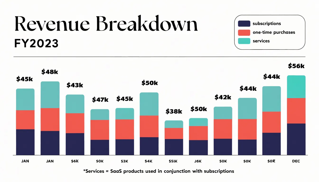
Stacking order matters for interpretation. Placing the largest or most stable segment at the base creates a consistent visual foundation, while smaller or more volatile segments sit at the top where changes are easier to notice. Combined with a clear legend and consistent color coding across views, stacked bars show where sales come from and how that composition shifts over time.
Pie Charts
Pie charts show how a total is divided into parts, making them well suited to static composition metrics such as market share and sales allocation. When a sales leader needs to show what portion of total revenue each product category, region, or channel contributes, a pie chart immediately conveys the relationship between each slice and the whole: a slice occupying a quarter of the circle represents a quarter of total sales, without requiring axes or scales.
Keep the number of slices to a practical ceiling of five to seven categories; beyond that, slices become too thin to distinguish. Group categories with negligible shares into a single ‘Other’ slice to preserve the total while keeping the main distribution visible. Ordering slices by size, typically clockwise starting from twelve o’clock, lets readers rank contributions and draws attention to the largest segments first.
Place slice percentages or absolute revenue figures directly on or beside each wedge so readers do not need to estimate angles, and anchor the chart with a title stating the measurement period and metric. Because stacked bar or line charts handle multi-period changes better, pie charts work best when the underlying total and mix are relatively stable and the goal is a snapshot of allocation.
Area Charts
An area chart fills the space beneath a line graph with a shaded color, turning a trajectory into a visual measure of volume. While the line’s height marks the value at any given point, the shaded region beneath it gives that value visual weight, communicating magnitude before viewers read a single number.
This shading makes area charts effective for tracking cumulative totals across consecutive quarters. As each period builds on the last, the filled region expands, showing how individual quarters accumulate into an annual figure. A sales team reviewing Q1 through Q4 can watch the area grow quarter by quarter to gauge momentum and pacing, while an underperforming quarter stands out as a sudden flattening of the band.
Area charts also support long-term trend analysis by placing many periods side by side without visual clutter, guiding the eye along seasonal patterns, plateaus, and inflection points. Stacked variations show how multiple product lines or regions combine into one total, with each band contributing its share of the overall envelope. The format works best for metrics centered on volume and accumulation—such as revenue totals, units sold, and pipeline value—anchored by a zero baseline and a restrained color palette.
Waterfall Charts
Waterfall charts bridge top-line revenue and the bottom line by showing each contributing factor as a sequential column that starts where the previous one ended. The chart opens with a full-height bar for gross revenue. Subsequent floating columns represent individual deductions or additions—such as discounts, product returns, chargebacks, and operating costs—at the cumulative level reached by prior columns. Viewers can trace exactly how much of the gross figure is consumed at every stage toward net income.
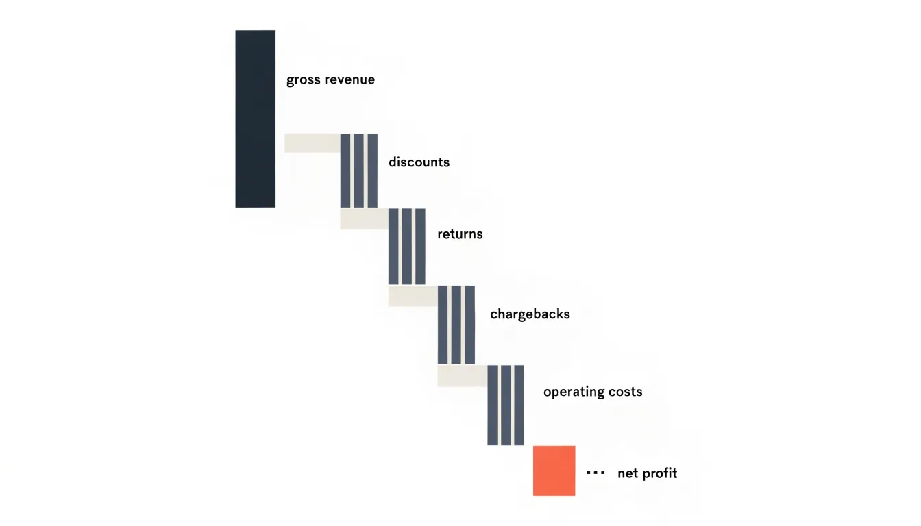
Color coding does much of the explanatory work: increases typically appear in one shade, decreases in another, and subtotal or total columns in a third tone. This lets readers instantly separate gains from losses. Because each bar begins at the running total of its predecessors, the chart preserves the arithmetic logic of the income statement in a left-to-right sequence.
In sales and finance reviews, a waterfall chart clarifies why a strong revenue quarter produced a modest profit. Breaking the gap between gross and net into discrete, attributable steps shows where margin pressure originates and which deductions are growing fastest. Tracked across multiple periods, the structure highlights trends in specific cost categories to help focus improvement efforts.
Funnel Charts
Funnel charts show how deals move through sequential pipeline stages, from lead generation through qualification, proposal, negotiation, and closing. Each stage appears as a horizontal or vertical band sized by deal count or total value, so the narrowing shape immediately shows where volume is lost as prospects advance. Mapping stages side by side turns raw pipeline data into a clear view of conversion momentum and bottlenecks.
The funnel chart’s primary strength is surfacing drop-off points. A steep contraction between stages signals where prospects are abandoning the buyer journey. A sharp drop between lead generation and qualification might point to poorly targeted marketing, while a squeeze between proposal and negotiation could indicate pricing concerns or weak competitive positioning. Sales managers can use this diagnostic view to target the specific stage needing improvement rather than applying generic fixes across the pipeline.
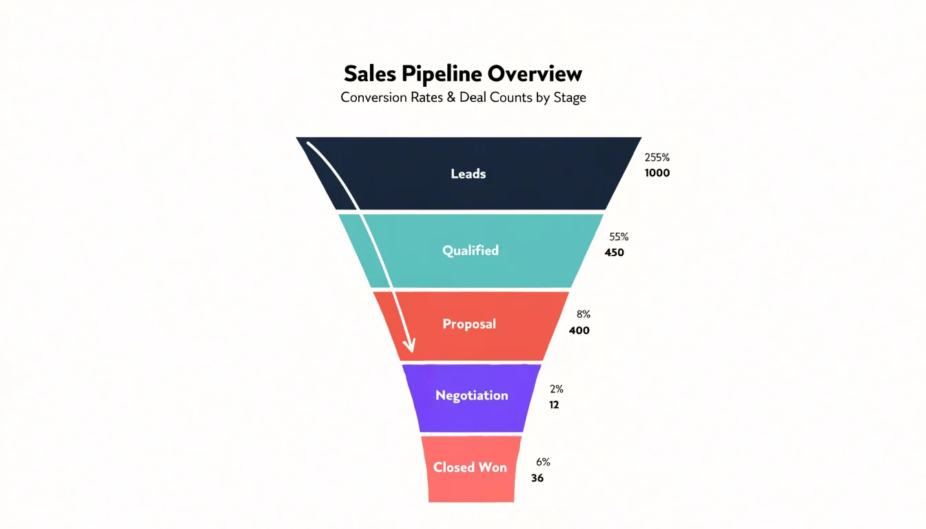
Funnel charts also support revenue forecasting and performance benchmarking. Because each band can display deal counts, conversion rates, or monetary value, teams can compare the current period against historical norms, align marketing and sales leadership on lead flow, and spot stalls during weekly pipeline reviews.
Scatter Plots
A scatter plot places one numerical variable along the horizontal axis and another along the vertical axis, plotting each observation as a single point at their intersection. In sales, this is ideal for examining how two measures move together across deals, products, or time periods. Plotting unit price against units sold, for example, turns each transaction or product line into a dot to reveal whether higher prices align with lower volumes, whether discounts cluster in a specific region, or whether the relationship is weak.
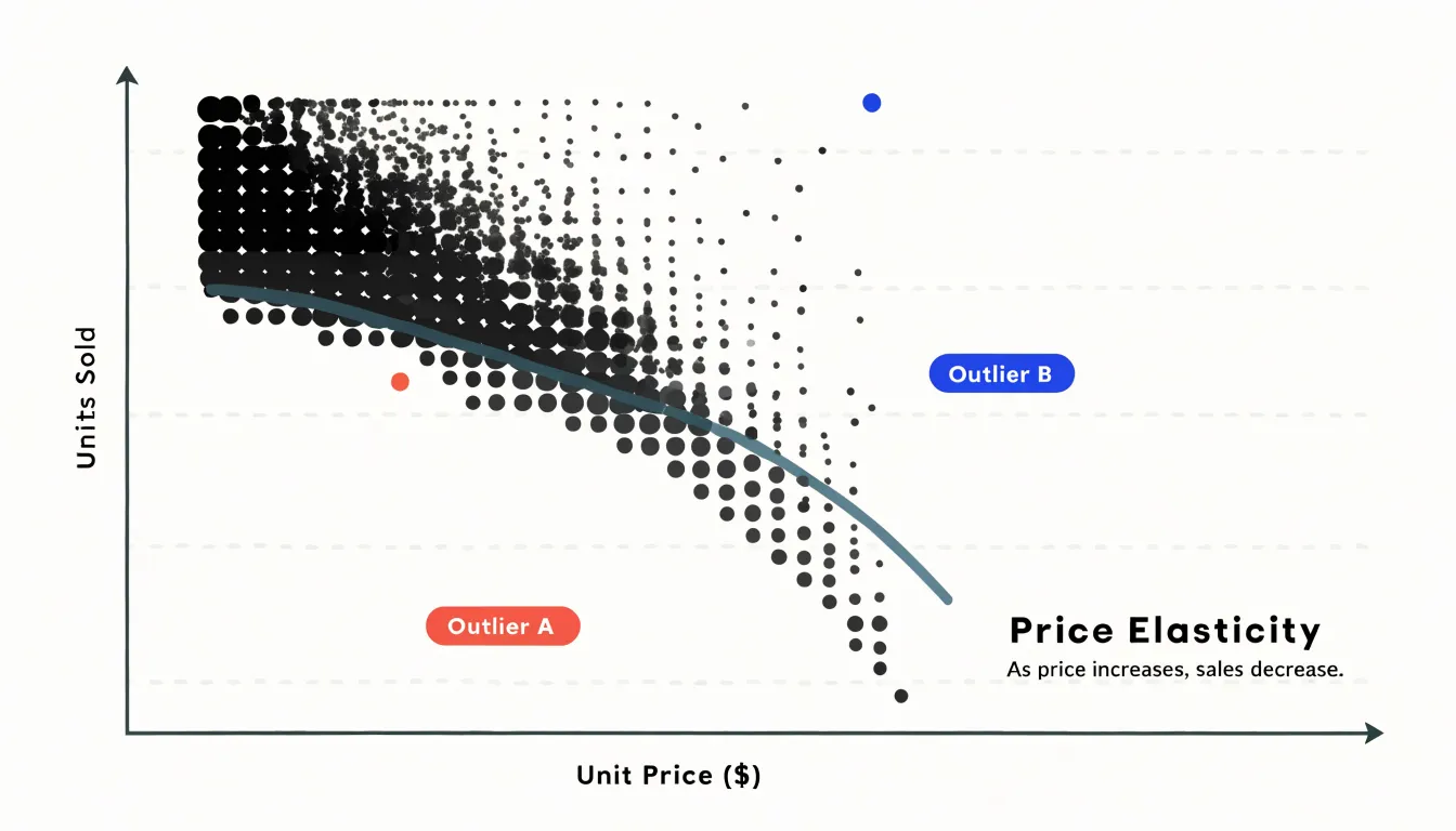
This approach reveals relationship patterns that summary tables hide. A tight downward band of points suggests a consistent negative relationship between price and volume (price elasticity). A looser cloud with wide vertical spread at the same price point indicates that other factors—such as region, promotion, or customer segment—are influencing volume. Outliers also stand out clearly: a high-price product selling unusually well, or a deep discount that failed to move units, appears far from the main cluster and invites investigation.
Similarly, plotting discount percentage against units sold shows whether incremental discounts produce steady gains or flatten beyond a certain threshold. Adding a trend line or coloring points by category sharpens these readings. Because scatter plots preserve every individual observation, they work best with moderate data volumes and careful axis scaling.
Heat Maps
Heat maps translate sales volume into color-density gradients so teams can spot peak activity at a glance. On a geographic heat map, regions are shaded by revenue or order counts; the darkest markets stand out as top performers while lighter zones reveal underdeveloped territory. Sales leadership can use this hierarchy to allocate field resources, plan regional campaigns, and spot expansion opportunities without scanning spreadsheet rows.
Applied to time, day-by-hour grids show when customers are most active. Retailers shade cells by transaction counts to expose lunchtime rushes, weekend surges, and quiet weekday afternoons, helping store managers schedule staffing and marketing teams time promotions. In e-commerce, hourly heat maps reveal when visitors convert most readily and when cart abandonment climbs.
Stacking color grids by location or season also lets analysts see how peak periods shift across markets and whether a promotion moved the needle in a given region. To ensure genuine patterns emerge rather than noise, analysts should aggregate data at sensible intervals, pair color intensity with clear legends, and use color-blind accessible palettes.
Combo Charts
Combo charts solve the scaling problem that occurs when two related metrics live on very different numeric scales—such as sales volume in dozens or thousands of units versus revenue in tens or hundreds of thousands of dollars. Plotted on a single axis, the smaller series flattens into a nearly invisible line along the bottom. A combo chart fixes this by pairing a bar series with a line series and assigning each to its own vertical axis within the same frame.
Typically, bars represent sales volume to give it a countable presence, while a line traces revenue as a continuous trend across weeks, months, or quarters (though the reverse also works depending on desired emphasis). Sharing a horizontal time axis invites direct comparison: rising bars paired with a dipping line signal discounting or a shift toward lower-priced products, while steady bars against a climbing line point to rising average order values.
To keep a dual-axis structure legible, limit the chart to two or at most three series, color-code each axis to match its series, label both y-axes with their units, and include a clear legend.
Histogram Charts
Histogram charts study price point distribution by grouping continuous transaction data into frequency bins. Each bar represents a price range, and its height shows how many transactions fell within that range, turning a long list of individual sale amounts into a snapshot of where buyers concentrate their spending.
Setting bin boundaries at meaningful increments—such as ten or fifty dollars—creates a frequency count for each interval and exposes patterns raw figures hide. Sharp peaks highlight the prices that attract the most interest, while gaps with very few transactions often reveal upper thresholds customers resist crossing.
The overall shape of the distribution shows average spend ranges. A cluster leaning toward the lower end suggests buyers prefer entry-level pricing, a spread toward higher bins indicates comfort with premium purchases, and a central bulk sets expectations for typical order values.
In practice, marketers can position promotions near the most populated bins, and product teams can introduce bundles that bridge the space between two strong clusters. Comparing distributions across regions or time periods also reveals shifting buyer behavior: movement toward higher bins signals growing willingness to pay, while concentration in lower bins may point to pricing pressure or a changing customer mix.
Pareto Charts
A Pareto chart combines a descending bar chart with a cumulative percentage line to reveal how unevenly revenue is distributed across products. Bars are arranged from highest-revenue item on the left to lowest on the right, while the line tracks the running percentage of total revenue on a secondary axis, rising steeply through the first few bars and flattening as smaller contributors are added. Where the line crosses the 80 percent mark, viewers can see how few products account for the bulk of income—often confirming the 80/20 pattern after only a handful of items.
Building the chart requires ranking products by total revenue for a chosen period, calculating each product’s share, and plotting the cumulative shares alongside the bars. Sales teams use this view to focus account management, inventory planning, and promotion budgets on the few products that carry the business, while flagging the long tail of low contributors for review, bundling, or discontinuation. Because the chart is sorted, shifts in which products occupy the leading bars across periods easily signal changes in demand or mix. Grouping minor items into an ‘Other’ category and clearly labeling the cumulative line keeps the chart readable.
Treemaps
A treemap turns a product portfolio into a single nested picture using rectangles sized in proportion to each product, category, or region’s sales volume. Larger boxes represent bigger revenue contributors, handling dozens or hundreds of items in a bounded space without the sprawl of a long bar chart or the clutter of a multi-slice pie chart. For hierarchical sales data—such as product lines containing subcategories and individual SKUs—outer rectangles group related items while inner rectangles break them down further.
Color adds a second dimension to encode revenue growth or decline. Applying a color intensity scale lets deep, saturated tones mark fast-growing products and muted or cool tones mark flat or shrinking ones. Combining size and color reveals portfolio dynamics at a glance: a large box in a weak color signals a core product losing momentum, while a cluster of small, intensely colored boxes points to emerging winners. This makes treemaps efficient for dashboards and quarterly reviews where managers must decide whether to defend a high-volume category or invest in a fast-growing niche.
Executive Dashboards
Executive dashboards combine multiple chart types into a single view for rapid strategic decisions. Start by selecting core KPIs—such as revenue, growth rate, pipeline coverage, average deal size, and win rate—and pairing each with its best-suited chart form: a line chart for revenue trends, a bar chart for regional or product comparisons, a gauge or bullet chart for target attainment, and a waterfall chart for decomposing revenue changes. Each visual should answer a specific leadership question without requiring further navigation.
Place the most critical KPIs at the top left and arrange supporting charts in descending order of importance. Group related metrics—sales performance, pipeline health, and revenue composition—into distinct clusters, and apply consistent color semantics across all charts: one color for actuals, another for targets, and a neutral palette for context, avoiding decorative elements.
To make the dashboard an interactive decision tool, add filters for time period, region, product, and sales team. Use hover tooltips for exact values and comparisons, and click-through actions to link to detailed reports. Keep the default view focused on the most recent quarter or year-to-date performance against targets and prior periods, constrained to a single screen with large fonts for headline metrics and brief text annotations for anomalies or milestones.
Frequently Asked Questions
What is the best chart for showing revenue trends over time?
Line graphs are the default choice for tracking revenue trends because they treat time as a continuous dimension and reveal the shape of change. They are especially effective for annual comparisons and for exposing seasonality when monthly revenue is plotted along a horizontal time axis.
When should I use a bar chart for sales data?
Bar charts provide a side-by-side view of sales performance across distinct categories, such as product lines, sales representatives, or geographic territories. They are useful for comparing total revenue, units sold, or average deal size because readers can judge relative performance by bar length.
How many slices should a pie chart have?
Pie charts should keep the number of slices to a practical ceiling of five to seven categories. Categories with negligible shares should be grouped into a single “Other” slice so the main distribution remains visible.
What is a waterfall chart used for in sales?
Waterfall charts bridge top-line revenue and the bottom line by showing each contributing factor as a sequential column that starts where the previous one ended. They help clarify why a strong revenue quarter produced a modest profit by breaking the gap between gross and net into attributable deductions or additions.
How do funnel charts show where deals are lost?
Funnel charts show how deals move through sequential pipeline stages, with each stage sized by deal count or total value. A steep contraction between stages signals where prospects are abandoning the buyer journey, helping managers target the stage that needs improvement.
What is a combo chart used for in sales reporting?
Combo charts solve the scaling problem when two related metrics live on very different numeric scales, such as sales volume versus revenue. They typically pair a bar series with a line series and assign each to its own vertical axis, while limiting the chart to two or at most three series for legibility.
Tony Astor
Tony writes about data visualization and the tools people use to build charts and dashboards. More about Data Illustrator