Best Charts for Reports: What to Use and Why
 By Tony Astor ·

Best Charts for Reports
Bar charts compare category values using bar length on a common baseline; line charts show trends over time; pie charts show parts of a whole; histograms display distributions across bins; scatter plots reveal relationships between two variables; and waterfall charts trace how a starting value reaches an ending value through gains and losses.
Table of Contents
Bar Chart
Bar charts translate category-to-value relationships into lengths that the eye can compare with remarkable precision. Because each bar stands on a common baseline, the relative size of one category against another becomes immediately legible without requiring the reader to decode angles, areas, or color gradients. This is why bar charts shine when a report needs to show, at a glance, which region sold the most, which product line underperformed, or how survey responses distribute across a fixed set of options. The discrete nature of bars maps naturally onto discrete categories, keeping the visual grammar aligned with the data structure.
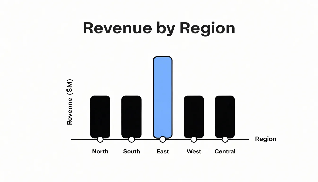
Ordering categories thoughtfully is one of the most consequential choices in building a bar chart:
- By value (descending or ascending): Creates a clear visual ranking that helps readers spot the top and bottom performers instantly.
- Alphabetically: Serves situations where readers need to locate a specific category quickly, such as a lookup table of departments.
- By natural sequence: Grouping by months or age bands preserves the logic of the underlying variable.
Whichever approach you take, keep the order consistent across related charts in the same report so readers can track categories from one figure to the next.
Orientation deserves equal attention. Vertical bars, often called column charts, work well when category labels are short and the number of categories is moderate. Horizontal bars become the better choice when category names are long, since labels can run along the left edge without rotation or truncation. Horizontal layouts also accommodate many categories by allowing the chart to grow downward, and they make value comparisons easier when categories are ranked from top to bottom. Time-based comparisons often suit vertical bars, while ranked lists of named entities typically read more naturally in horizontal form.
Line Chart
A line chart shows how a value changes over time by connecting individual data points with a continuous line. This turns a series of measurements into a visible trajectory, so readers can quickly see whether a metric is rising, falling, plateauing, or fluctuating. It works best when the data is continuous and the intervals on the horizontal axis follow a chronological order, such as days, weeks, months, or years. A steady upward slope signals growth, a sharp dip draws attention to an anomaly, and a long flat stretch suggests stability.
Multiple lines can share the same axes to show how different categories move relative to one another, for example revenue across several product lines over a year. The spacing between the lines reveals gaps and convergences, giving readers a sense of relative performance without extra explanation. Markers at each data point can help when the intervals are irregular or when the exact values matter.
Common mistakes undermine these strengths:
- Misleading axis scaling: Starting the vertical axis at a value far from zero, or skipping intervals, can exaggerate small changes into dramatic swings.
- Inconsistent horizontal spacing: Mixing months and quarters on the same axis distorts the time relationship.
- Too many lines: Overcrowding makes the chart cluttered and hard to follow.
A clear title, labeled axes, and honest scaling keep the chart trustworthy and make the trend the focus.
Pie Chart
Pie charts show how a single total divides into component parts, giving readers an immediate sense of proportion. Each slice represents a category’s share of the whole, and the entire circle equals 100%. This makes the format well suited to simple percentage distributions in reports, such as the breakdown of a budget by department, market share among leading competitors, or survey responses across a handful of answer options.
Clarity depends on strict limits:
- Restrict the chart to five slices or fewer: Beyond that threshold, slices become narrow wedges that are difficult to label and compare; readers cannot reliably judge whether one small slice is larger than another. Group minor categories into a single combined slice to preserve the overall picture.
- Order slices logically: Typically run them from largest to smallest, beginning at the twelve o’clock position so readers can scan the distribution consistently.
- Label directly: Mark each slice with its category and percentage, and consider adding the underlying value where precision matters.
- Avoid distortion: Skip three-dimensional effects and exploded slices, which warp the geometry and undermine comparisons.
When the data features a modest number of categories, percentages that total 100, and a message centered on proportion rather than fine-grained comparison, the pie chart earns its place in a report.
Histogram
A histogram takes a set of continuous quantitative measurements and sorts them into a series of adjacent bars, each representing a defined range of values known as a bin. The width of every bin covers a fixed interval along the horizontal axis, and the height of the bar records how many observations fall within that interval. This turns a long list of raw numbers—such as response times, transaction amounts, or customer ages—into a compact visual summary of where values cluster and where they are sparse.
By choosing sensible bin boundaries, the histogram collapses thousands of distinct values into a manageable number of categories while preserving the overall pattern. Readers can see the central tendency at a glance, since the tallest bars typically sit near the middle of the distribution. They can also spot skewness: a long tail stretching to the right or left reveals that a subset of observations lies far from the main group. Multiple peaks may indicate that the data combines two distinct populations.
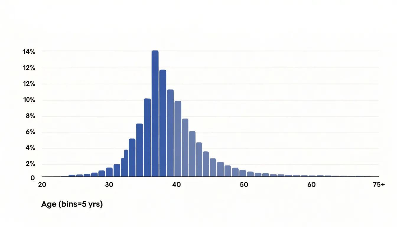
Gaps between bars show ranges where no observations occurred, and gradual slopes show how quickly counts rise or fall across the scale. These features help analysts judge whether a process is stable, whether outliers deserve investigation, or whether a distribution matches an expected model. The choice of bin width affects the picture, with narrow bins exposing fine detail and wide bins smoothing noise.
Scatter Plot
A scatter plot places one variable along the horizontal axis and another along the vertical axis, drawing a single dot for each observation where its two values intersect. When the dots drift upward from left to right, the two variables move together in a positive correlation; when they slope downward, one tends to rise as the other falls, indicating a negative correlation. A cloud of dots with no discernible slope suggests the variables are largely independent. Because the eye can absorb hundreds or thousands of points at once, scatter plots work especially well with large dataset pairs that would be unreadable in a spreadsheet.
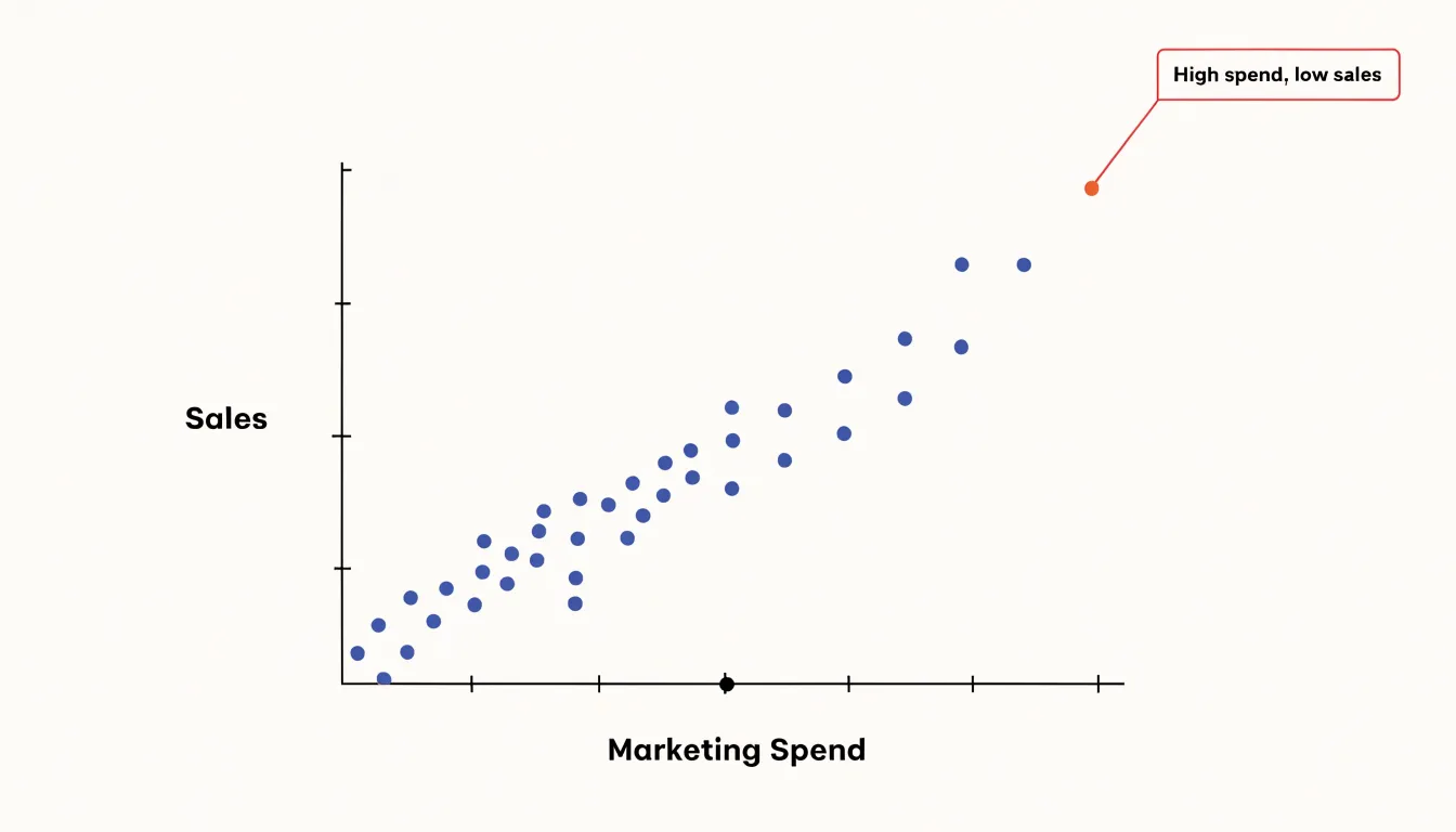
Outliers stand out clearly in this format. A point sitting far from the main cluster may represent a data-entry error, an unusual case, or a genuinely different subgroup worth investigating, flagging it in a way summary statistics often hide.
Scatter plots also help analysts think carefully about causation. A tight correlation can prompt the question of whether one variable drives the other, but the chart itself only shows association. Still, the shape of the relationship offers clues: a linear band, a curved pattern, or distinct clusters each tells a different story about how the variables interact, letting readers judge whether further investigation into cause and effect is warranted.
Area Chart
An area chart fills the space between a trend line and the horizontal axis. Where a simple line chart traces the path of a value, the shaded area beneath it represents the accumulated quantity behind that path, so the reader sees both the direction of movement and the volume it reflects. This makes area charts a natural fit for reporting cumulative totals over time, such as revenue building across quarters, registered users accumulating month over month, or total hours logged by a team throughout a project cycle. The slope of the upper edge communicates the rate of change, while the height and bulk of the filled shape convey the magnitude reached at each stage.
The format works especially well for continuous data recorded at regular intervals, where the fill reinforces the sense of an ongoing, unbroken process. Reports that show growth trajectories, seasonal peaks, or the buildup of a running total benefit from this dual reading of shape and substance. Designers can strengthen the effect by labeling key values along the top edge, using a single restrained color, and keeping gridlines light so the filled area stays dominant. Stacked variants extend the same logic to part-to-whole totals, letting each segment’s contribution appear as a band within the overall silhouette.
Stacked Bar Chart
A stacked bar chart compares subgroups within categories by stacking sub-segments on top of one another. The total height of the bar represents the overall value for the primary category, while each segment shows the contribution of a specific subgroup. This dual view allows readers to compare total values across categories and examine internal composition at the same time.
For instance, a report might display revenue by region, with each bar representing a region and segments showing revenue from different product lines. Viewers can quickly see which region has the highest total revenue and how the product mix varies between them. Other common uses include budget allocation by department and expense type, or survey responses by demographic group and answer choice.
However, interpreting stacked bars requires care. While the bottom segment is easy to compare across bars because it shares a common baseline, segments higher up do not align on a consistent scale. Comparing the sizes of individual subgroups across categories can be challenging unless the segments are ordered consistently or the differences are large. Consequently, stacked bar charts work best when the primary goal is to compare totals and get a general sense of composition, rather than to make precise comparisons of individual sub-segments.
Bubble Chart
A bubble chart extends the scatter plot by encoding a third variable through the size of each circle. The position of each bubble communicates two numbers (x-value and y-value), and its radius or area communicates a third, allowing a single chart to display data triples across a set of items such as products, regions, or business units.
Consider a report examining business performance across markets. Cost can sit on the horizontal axis and revenue on the vertical axis, giving each market a clear position in terms of efficiency and scale. Market share then becomes the size of the bubble. A large bubble high on the revenue axis represents a market with strong sales and a substantial share, while a small bubble far to the right indicates high cost with limited revenue and modest presence.
The size dimension works best when circle areas, rather than diameters, are scaled to the values, since the human eye tends to underestimate differences in area when diameters grow linearly. Labels or a legend help readers map bubble sizes to actual figures, and a restrained color palette keeps attention on the size and position of each circle. Used with a manageable number of bubbles, the chart turns a complicated multi-variable comparison into one coherent view.
Heat Map
A heat map turns a matrix of numbers into a field of color, letting readers absorb density and intensity before reading a single value. Rows and columns represent two categorical dimensions—such as products and regions, or hours and weekdays—and each cell is filled with a shade drawn from a color gradient. Deeper or warmer tones mark higher values, while lighter or cooler tones mark lower ones. Clusters of dark cells reveal hot spots where activity concentrates, and diagonal or block formations expose correlations between categories.
Because a well-designed gradient leads the eye naturally toward the most important cells, high-density zones and anomalies stand out immediately even in a dense matrix. A single unexpected dark or pale cell interrupts the surrounding rhythm and invites investigation, allowing reviewers to locate outliers first and then examine the underlying figures rather than reading numbers row by row.
Sequential gradients suit data that runs from low to high, while diverging palettes help when values fall on either side of a meaningful midpoint such as zero or an average. Legible contrast, sensible binning, and a clear legend keep the map honest and readable.
Waterfall Chart
A waterfall chart shows how a starting value arrives at an ending value through a series of intermediate changes. Each category of change appears as a floating bar positioned along a vertical axis, stepping up or down in sequence to reflect gains and losses. The first bar typically represents the opening balance, the middle bars show individual positive and negative movements, and the final bar resolves into the closing total. Because every floating bar begins where the previous one ended, the reader can follow the cumulative effect of each adjustment without mental arithmetic.
This structure is especially useful in financial and operational reporting:
- Financial results: Break a net income figure into contributing components such as sales growth, price changes, currency effects, and one-off expenses.
- Operational metrics: Decompose headcount changes, capacity shifts, or budget variances into the discrete events that produced the final number.
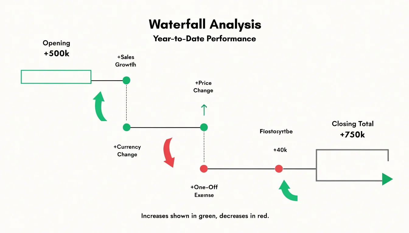
Large steps draw the eye to the most significant drivers, while small or offsetting movements recede into the background. Color coding conventionally distinguishes increases from decreases, and connecting lines between bars reinforce the idea of a running total, making the chart read like a ledger translated into geometry.
Funnel Chart
A funnel chart represents a linear, sequential process as a series of stacked, progressively narrowing horizontal bars. Each stage corresponds to a step in the journey, and the width of each bar reflects the number of people or units that reach that point. This shape makes it immediately clear where volume is lost, which is why funnel charts are a staple in reports covering sales pipelines, signup flows, checkout sequences, and user onboarding.
By labeling each segment with both the raw count and the percentage retained from the previous step, a report can show exactly how many prospects advance from lead to qualified opportunity to closed deal, or how many new users progress from account creation to first key action to sustained engagement.
When one bar narrows sharply relative to the bars around it, that bottleneck step becomes an obvious candidate for investigation. Authors can annotate the funnel with drop-off percentages between stages to direct attention to the single step where the largest absolute or proportional loss occurs. Funnel charts work best when participants pass through ordered steps without skipping ahead, and with a modest number of stages—typically four to seven—paired with clear stage definitions and consistent time windows.
Box Plot
A box-and-whisker plot, or box plot, condenses the distribution of a dataset into a compact visual summary for quick statistical comparison across multiple groups:
- Central box: Spans the interquartile range (IQR) from the first quartile (Q1, the 25th percentile) to the third quartile (Q3, the 75th percentile), capturing the middle 50% of the data. A longer box means greater variability.
- Median line: Sits inside the box at the 50th percentile to mark central tendency.
- Whiskers: Extend from the box to the most extreme data points within 1.5 times the IQR from the quartiles, showing the range of typical data.
- Outliers: Points beyond the whiskers are plotted individually, flagging unusual or extreme values.
When comparing groups side by side, differences in medians, IQRs, and outlier patterns become apparent at a glance. Box plots are robust to non-normal distributions and are less affected by extreme values than mean-based summaries, making them well suited for exploratory data analysis and reports where space is limited.
Sankey Diagram
A Sankey diagram maps the movement of volume through a connected system, drawing each transfer as a band whose width is proportional to the quantity flowing. Readers can compare the relative size of every stream at a glance, tracing where resources enter, how they split across branches, and where they finally accumulate.
Common applications include:
- Energy and sustainability reporting: Follow input fuels through conversion stages to final consumption, showing how much energy is lost as heat and how much reaches end users. Grid operators use the same structure to illustrate power transfers between regions, while sustainability teams apply it to material and waste flows.
- Customer journey analysis: Trace a cohort from first touchpoint through the channels and pages they visit, splitting where audiences diverge and converging where they convert or drop off. This reveals which paths carry the most traffic and where volume leaks away—information a funnel chart alone tends to flatten.
Every node and link needs a clear name, and figures or percentages help readers verify what the band widths imply. Color can distinguish major flow categories, though palettes should stay restrained to avoid clutter.
Dashboard
A dashboard works best when it treats its collection of charts as a single composition answering an executive summary, rather than a loose pile of images. It usually opens with the single most important metric or trend in the top-left position where the eye lands first, presented as a large number or a clean line chart. Supporting visuals then explain why that headline figure looks the way it does—a breakdown by segment, a comparison against target, or a distribution showing where variation comes from. No two panels should repeat the same information.
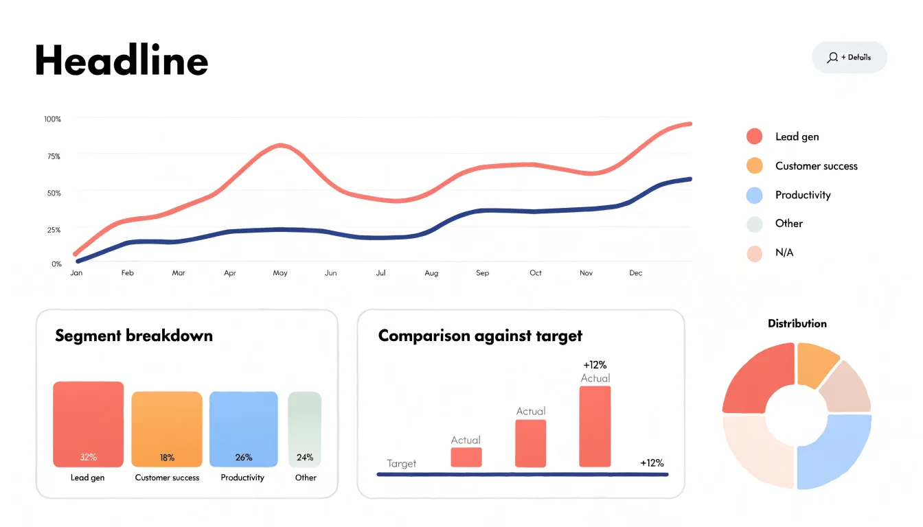
Visual hierarchy and layout keep the composition readable:
- Size and weight: The primary chart should occupy the most space, while secondary panels stay smaller and quieter.
- Consistency: Shared axes where comparisons matter, consistent scales, and a restrained palette keep the viewer from re-learning how to read each panel.
- Logical grouping: Placing related views near one another (such as all revenue charts in one row) reduces scanning effort and lets viewers move from overview to detail.
- Spacing and alignment: Generous margins, aligned edges, and uniform gaps let the data stand out.
- Actionable titles: State the takeaway directly rather than just naming the metric, so a reader can absorb the story by skimming.
Limit the dashboard to roughly five to seven panels so attention does not fragment. Finally, test the layout with a real audience, watch where their eyes go, and refine the arrangement until the intended message lands first.
Frequently Asked Questions
What is a bar chart best for in reports?
Bar charts are best for showing category-to-value relationships, such as which region sold the most, which product line underperformed, or how survey responses distribute across fixed options. Their common baseline makes relative category sizes easy to compare without decoding angles, areas, or color gradients.
How many slices should a pie chart have?
A pie chart should be restricted to five slices or fewer, because beyond that threshold slices become difficult to label and compare. Minor categories can be grouped into a single combined slice to preserve the overall picture.
When should I use a histogram?
Use a histogram for continuous quantitative measurements, such as response times, transaction amounts, or customer ages. It sorts values into adjacent bins so readers can see where values cluster, where they are sparse, and whether the distribution is skewed.
How can I tell if a scatter plot shows correlation?
Dots drifting upward from left to right indicate a positive correlation, while a downward slope indicates a negative correlation. A cloud of dots with no discernible slope suggests the variables are largely independent, and the chart itself only shows association, not causation.
What is a stacked bar chart best for?
A stacked bar chart compares subgroups within categories by stacking sub-segments on top of one another, with total bar height showing the overall value and segments showing composition. It works best when the primary goal is comparing totals and getting a general sense of composition, rather than making precise comparisons of individual sub-segments.
How many panels should a dashboard have?
A dashboard should be limited to roughly five to seven panels so attention does not fragment. It should open with the single most important metric or trend in the top-left position, with supporting visuals explaining why that headline figure looks the way it does.
Tony Astor
Tony writes about data visualization and the tools people use to build charts and dashboards. More about Data Illustrator