Best Charts for Presentations (With Design Tips)
 By Tony Astor ·
Best Charts for Presentations (With Design Tips)
Bar charts compare discrete categories, line graphs show change over time, pie and donut charts show parts of a whole, and scatter plots reveal relationships between two variables. Stacked bars, area charts, waterfalls, funnels, radar, gauge, and treemap charts each suit specific data stories. Choose the chart type that matches your message, then simplify by removing clutter.
Table of Contents
Bar Charts
Bar charts are the workhorse of presentation visuals, and they earn that reputation because they make discrete comparisons immediately legible. A horizontal or vertical bar chart assigns each category its own bar, letting the audience read relative size at a glance without mental arithmetic. When the goal is to show how one group stacks up against another, the bar chart removes ambiguity and directs attention to the differences that matter.
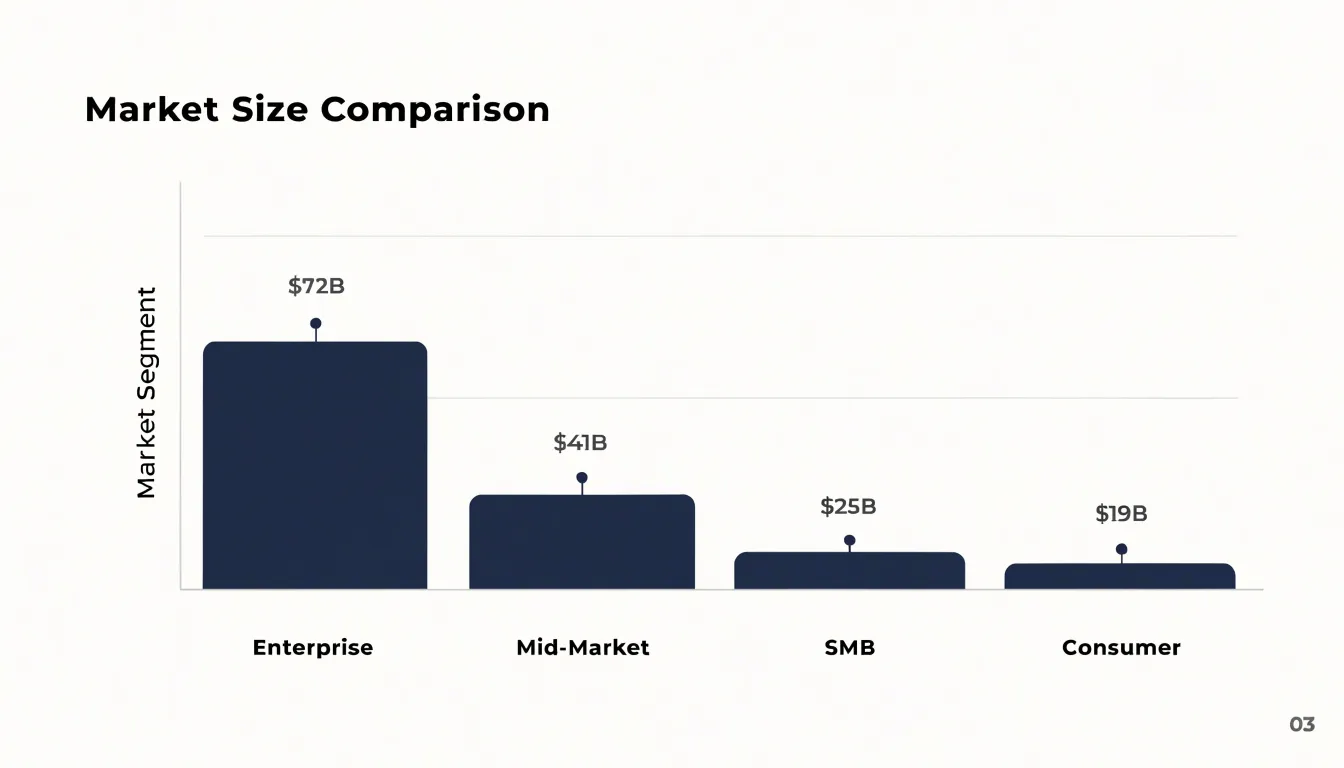
The orientation choice shapes how the chart reads. Vertical bar charts, sometimes called column charts, suit a small number of categories with short labels and a natural left-to-right flow, such as quarterly results or age brackets. Horizontal bar charts shine when category names are long, when there are many categories, or when the labels would otherwise crowd the axis; they let labels sit flat and readable at the left edge. Either orientation keeps the comparison honest, since the shared baseline makes bar length the single visual cue audiences use to judge value.
Ordering is where many bar charts gain or lose impact. Sorting bars by value, descending or ascending, turns a jumble of categories into a clear ranking that answers the obvious question before it is asked. Grouped ordering, such as alphabetical or chronological sequence, works when the category order itself carries meaning for the audience. Placing the most important or largest bar first anchors the eye, and keeping the number of bars modest prevents the chart from becoming a wall of thin lines. Consistent bar width, generous spacing, and data labels at the bar ends round out a presentation-ready chart that lets differences speak plainly.
Stacked Bar Charts
Stacked bar charts let a presenter show several sub-groups bundled inside each main category, so the audience sees both the overall size of each category and how it breaks down. The format works best when the composition of each bar matters as much as the total, such as quarterly revenue split by product line or survey responses segmented by age group. Keep in mind that viewers read the total length of each bar as the absolute figure and the colored segments as relative shares, so make both readings easy. Label the axis with clear totals, and place segment percentages or values inside each block when the numbers are central to your message.
Clutter creeps in quickly with stacked bars. Limit each bar to three or four segments; beyond that, colors become hard to distinguish and legends grow unwieldy. Order segments consistently across every bar, placing the largest or most important group at the base of the stack so it is easiest to compare. Use a restrained palette with clear contrast between adjacent segments, and lean on direct labels rather than a crowded legend whenever space allows. For slides, favor horizontal stacked bars for long category names and keep the chart area uncluttered by stripping gridlines and decorative elements.
The biggest pitfall is confusing absolute and relative totals. When segment sizes vary, viewers may misjudge proportions because only the bottom segment shares a common baseline. A 100% stacked bar resolves this by normalizing every bar to the same length, which emphasizes composition and removes the absolute comparison entirely. Choose plain stacked bars when totals differ and those differences carry meaning; choose 100% stacked bars when the story is about share. State in the title which reading applies, so the audience knows whether to compare bar lengths or segment proportions.
Line Graphs
Line graphs are the tool of choice whenever a presenter needs to show how a value changes across a continuous span of time. Because the eye naturally follows a connected path from left to right, a line graph turns a sequence of data points into a story of movement: rising, falling, plateauing, or oscillating. This makes it ideal for growth trajectories, seasonal spikes, and sudden drops that would be harder to perceive in a table or a bar chart.
The horizontal axis should carry a consistent chronological interval—whether days, months, quarters, or years—so viewers can trust that the spacing between points reflects real elapsed time. Keep the vertical axis starting at zero when absolute magnitude matters, and label it clearly so the scale is never in question. Limit the number of lines on a single chart; three to five series is usually the practical ceiling before the plot becomes a tangle. When comparing multiple series, differentiate them with distinct colors and direct labels placed near the end of each line, which spares the audience from darting back and forth to a legend.
Mark significant events, campaign launches, or policy changes with a subtle vertical annotation so spikes and drops acquire context. Smooth or dashed line styles can distinguish actual recorded values from projections, giving viewers an honest sense of where certainty ends. Avoid plotting too many data points at fine granularity, since dense zigzags obscure the underlying trend; aggregating to weekly or monthly averages often communicates more clearly. Finally, keep gridlines faint and the data line prominent, and state the key takeaway in the slide title so the trend is understood at a glance.
Pie and Donut Charts
Pie and donut charts work best when the goal is to give an audience an immediate sense of how a whole breaks down into a few parts. A presenter showing market share, budget allocation, or survey results can use a circular chart to communicate the rough proportions in a single glance, since viewers intuitively read each slice as a fraction of the complete circle. The labels and percentages placed around or inside each segment reinforce that reading without requiring the audience to interpret axes or scales.
These charts perform well under tight constraints. Limiting a pie to about five slices keeps it legible from the back of a room and prevents the visual clutter that comes from many thin wedges. When data includes more categories, grouping the smallest values into a single “Other” slice preserves clarity. Slices should be ordered by size, usually starting at the twelve o’clock position and moving clockwise, so viewers can compare segments without hunting for the largest one. Values that are nearly identical are difficult to distinguish in a circle, so a bar chart often serves better when close comparisons matter.
The donut chart adds practical value for presentations through its open center. That empty space provides room for a headline figure, a short label, or an icon that anchors the chart’s message, such as total revenue or the number of respondents. Presenters can place the most important number directly in the middle, drawing attention to the overall context while the ring communicates the breakdown. The central callout also reduces the need for separate text boxes elsewhere on the slide.
Both formats suit slides that prioritize quick proportional insight over precise measurement. Designers should keep colors distinct and limited, label slices directly rather than relying on a distant legend, and reserve these circular charts for the moment when a simple share of a whole is the point of the message.
Scatter Plots
Scatter plots are the right choice when you need to show how two numerical variables relate to one another. Each dot on the plot represents a single data point, positioned according to its values on the horizontal and vertical axes. This simple structure lets an audience see patterns emerge from the data at a glance: whether values rise together, fall together, or show no clear relationship at all. When preparing a scatter plot for a presentation, begin by plotting each paired dataset as a dot and letting the overall shape of the cloud tell the story. A dense band running from lower left to upper right signals a positive correlation, while a band running the other direction indicates a negative one. A shapeless spread suggests the two variables move independently.
Clusters deserve explicit attention. When dots bunch together in distinct groups, they often point to meaningful subgroups within the data, such as different customer segments, regions, or time periods. Point these clusters out in your commentary, and consider using a slightly different color for each so the audience can follow without needing a legend-heavy explanation. Outliers matter just as much. A handful of dots sitting far from the main cloud can represent errors, exceptional cases, or the most interesting story in the dataset. Label only the few outliers that matter rather than naming every point.
Non-technical stakeholders benefit from restraint. Keep the plot uncluttered by removing gridlines that add noise, limiting the number of series to three or four at most, and using plain language in axis labels, such as ‘Monthly spend’ instead of ‘rev_per_acct_30d’. Avoid overplotting by reducing dot size or adding slight transparency when many points overlap. A single trend line, drawn lightly, can reinforce a correlation without implying more precision than the data supports. Finish with a short title that states the takeaway, for example ‘Higher engagement tracks with longer retention,’ so the audience reads the finding before they read the axes.
Area Charts
Area charts take the familiar line chart and fill the space beneath the line with color, turning a simple trajectory into a statement about magnitude. This shading transforms the chart from a record of direction into a representation of volume, so audiences read not only where a metric is heading but how much of it exists at any given moment. When the goal is to show growth in total terms — revenue accumulating over quarters, users stacking up across a year, hours logged month after month — the filled region communicates that weight instantly, without requiring viewers to translate a line’s height into a mental estimate of quantity.
What makes area charts particularly useful in presentations is their ability to carry multiple layers at once. Stack several series on top of one another and the uppermost boundary traces the combined total, while each colored band below reveals how individual components contribute to that whole. A marketing team might use this to show overall lead volume rising across four quarters while making visible that organic search, paid campaigns, and referrals each grew at different rates and shifted in relative share. The chart does double duty: it answers the executive question about cumulative growth and the operational question about which channels are driving it.
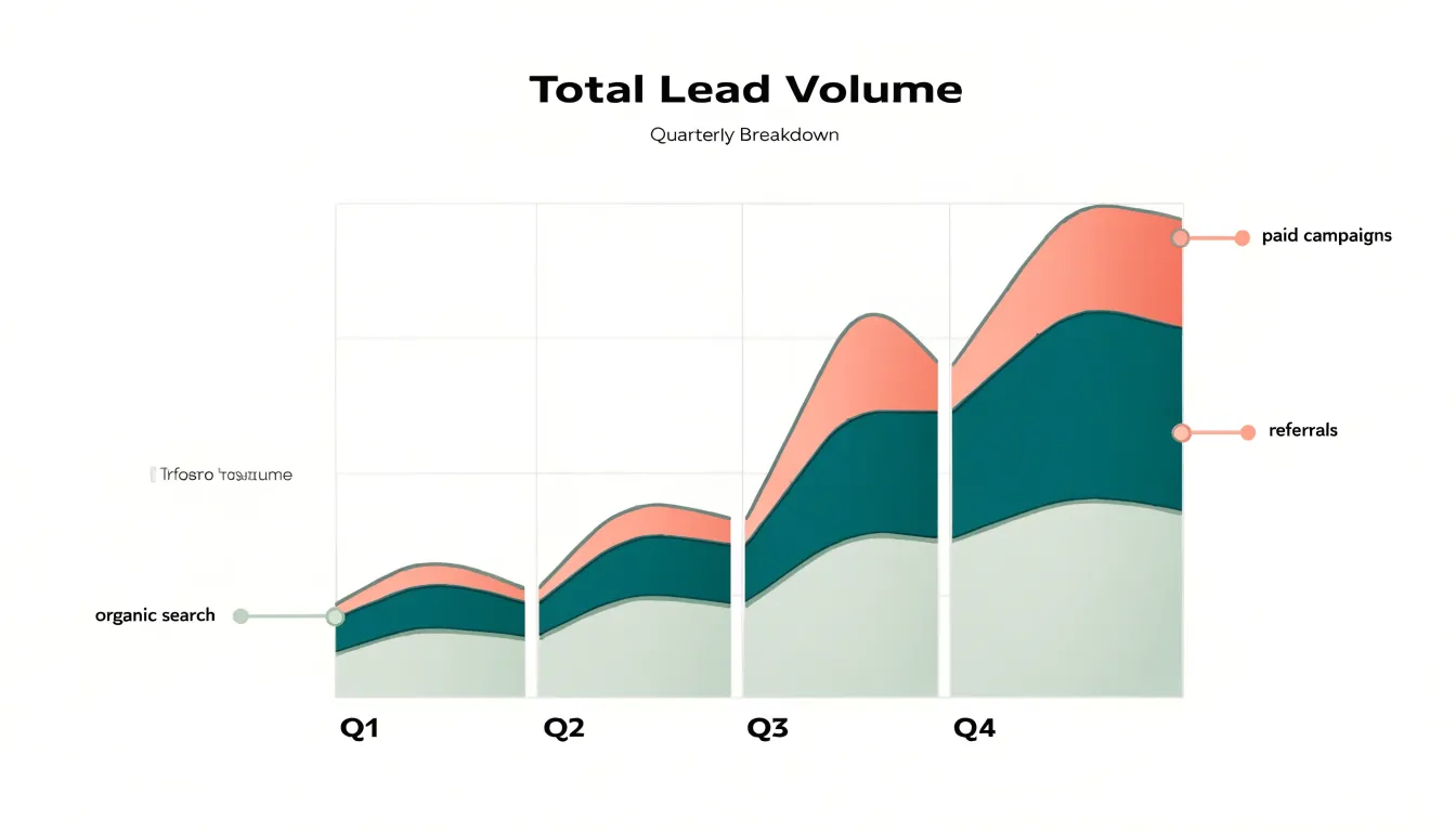
The format rewards extended timeframes. With a dozen or more data points across months or years, area charts reveal seasonal rhythms, inflection points, and the compounding effect of steady gains. Design choices matter here: keep the number of stacked layers modest, order them logically, and use a graduated palette so adjacent bands remain distinguishable. Light gridlines and clear axis labels keep the focus on the shaded shapes rather than the framework around them, letting the visual weight of the filled regions do the explanatory work for the audience.
Waterfall Charts
Waterfall charts are built for one specific job: showing how a starting figure travels through a series of positive and negative adjustments to arrive at a final result. Each category in the chart appears as a floating column, with its base resting on the cumulative total of everything before it. A revenue increase lifts the next column upward, a cost or deduction drops it downward, and the eye follows the staircase of gains and losses until the last bar lands on the net figure. Because the columns bridge from one running total to the next, viewers can see both the individual contribution of each item and the cumulative effect of all of them together.
This structure makes waterfall charts a natural fit for financial breakdowns and earnings reports. A typical example starts with gross revenue, subtracts cost of goods sold, operating expenses, and taxes step by step, and finishes with net income as a solid anchor bar at the end. Presenters can walk an audience through the bridge line by line, pausing on any bar that deserves discussion, without losing the thread of how the bottom line was reached. The same logic works for budget-versus-actual reviews, where each variance is a step between planned and realized figures, and for cash flow summaries that track how an opening balance becomes a closing balance.
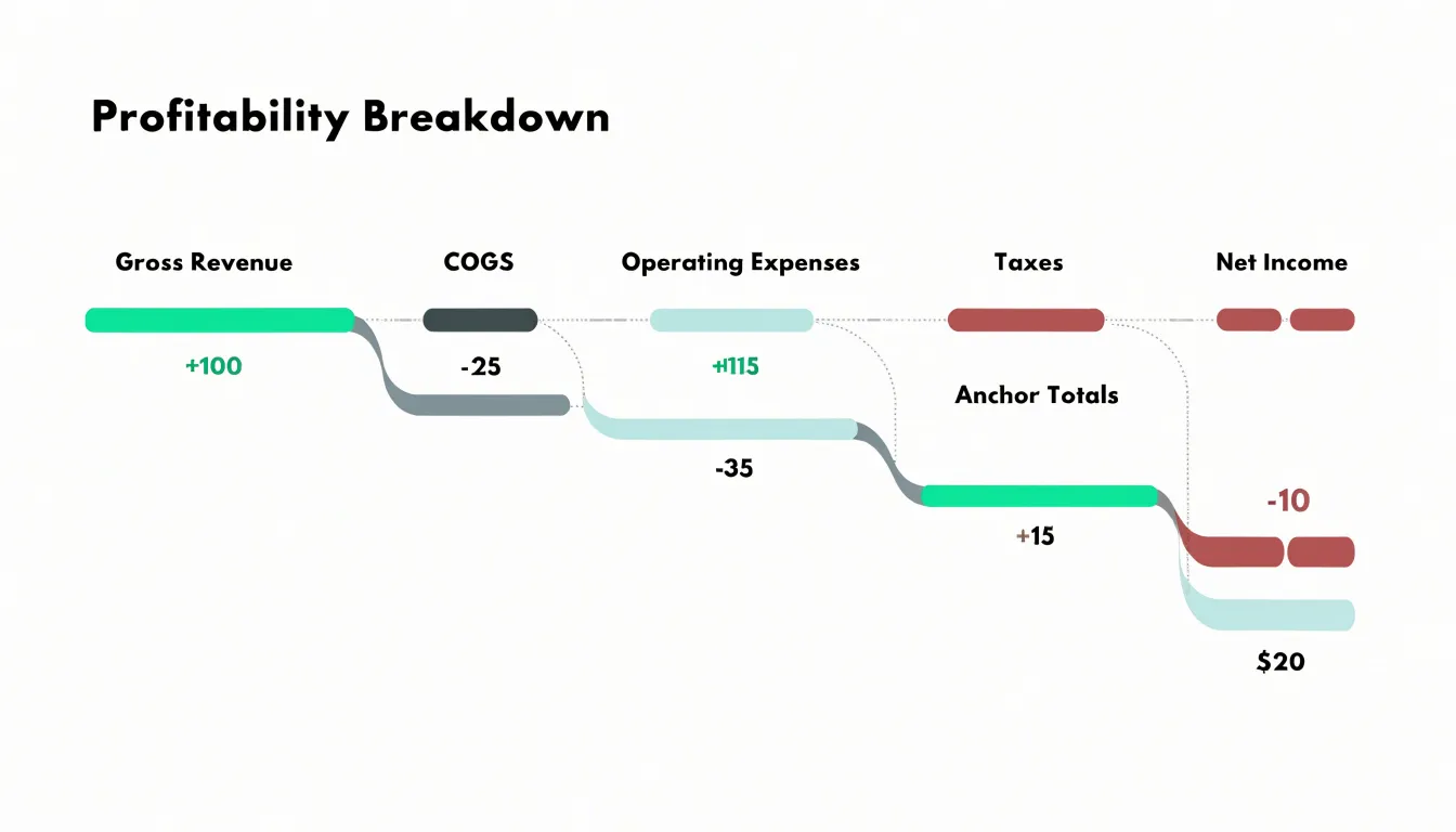
Design choices matter a great deal here. Color-code increases and decreases consistently, for example a calm green for gains and a muted red for losses, and use a neutral tone for the opening and closing totals so the anchors stand apart from the movements. Label each bar with its value, since precise figures are the point of this chart, and keep the category labels short enough to read at a glance. Order the steps in the sequence they actually occur, add connector lines between columns to reinforce the flow, and avoid cramming in so many items that the staircase becomes a staircase of noise.
Funnel Charts
Funnel charts earn their place in presentations whenever a process moves through sequential stages toward a single goal, with each stage narrowing the population that continues forward. Sales pipelines offer the classic example: leads enter at the top, then move through qualification, proposal, negotiation, and close, with the chart’s tapering shape making the overall health of the pipeline visible at a glance. The same structure works for user onboarding, where visitors progress from sign-up to activation, first key action, and retained use. Funnel charts are equally useful for mapping journeys such as application flows, donation processes, or customer support escalation paths, since any multi-step sequence with measurable transitions can be visualized this way.
The primary value of a funnel chart is diagnostic. By displaying the count or percentage at each stage, the chart directs attention to where the largest drop-offs occur. A steep narrowing between two stages signals a bottleneck that deserves investigation, whether that means a confusing form field, an unclear pricing step, or a follow-up that arrives too late. Presenters can use this visual evidence to prioritize process improvements, focusing effort where the loss is greatest rather than spreading resources evenly across every stage. Showing conversion rates alongside absolute numbers helps an audience weigh the relative cost of each gap.
Design choices should keep the funnel readable in a live presentation setting. Order stages top to bottom in true sequence, label each with both a name and a value, and keep the funnel limited to roughly five to seven stages so the shape stays legible. Color should emphasize the stages that matter most, and annotations calling out the sharpest drop-off turn the chart into a clear call to action. A brief note on the data source and time period builds credibility with the audience.
Radar Charts
Radar charts, sometimes called spider charts or web charts, display several quantitative variables measured on the same scale by plotting each variable along its own radial axis radiating from a central point. Each axis represents one performance factor, and the values recorded for a given item are connected across the axes to form a distinctive polygon. This makes radar charts a strong choice for presentations that need to evaluate multi-attribute datasets, such as skill assessments or product feature comparisons, where the audience must grasp the overall profile of an entity at a glance.
The most important requirement is normalization. Every axis should share the same scale, or at least a scale where equivalent distances carry equivalent meaning, so the shape of the polygon reflects real differences rather than artifacts of mismatched ranges. When axes are normalized, the resulting silhouette does its work intuitively: a balanced performer produces a broad, rounded shape, while one with concentrated strengths and gaps produces a spiky, uneven outline that immediately communicates a profile. This visual shorthand is why radar charts appear so often in competency frameworks, employee evaluations, and competitive product breakdowns.
For presentation use, keep the number of axes between five and eight; fewer produces an oversimplified shape, and more turns the chart into a dense thicket that audiences cannot parse. Label each axis clearly and position it consistently around the circle so comparisons across multiple slides remain stable. Overlaying two or three series, for instance a current state and a target state or two competing products, works well when each polygon uses a distinct outline and a light, translucent fill, letting viewers see where shapes overlap and diverge. Placing the chart alongside a short callout of the two or three most significant axis differences helps the audience move from impression to insight.
Gauge Charts
Gauge charts use a dial-style visual to show where a single metric currently sits relative to a predefined scale. The most familiar form is the speedometer: a semicircular arc marked with low, mid, and high zones, a needle pointing to the current value, and often a numeric readout in the center. In a presentation, this format works best when the audience needs an instant verdict on one number rather than a comparison across categories or a trend over time. A sales team tracking progress toward a quarterly revenue goal, a factory floor monitoring pressure inside a safe operating range, or a service desk watching average response time against an SLA can all convey status at a glance with a well-built gauge.
The design of the scale does most of the communicative work. Colored bands along the arc mark thresholds: green for on-target, amber for caution, red for critical. These zones should be defined before the chart is drawn and should reflect real business rules, such as a safety limit or a contractual target. Place the needle so it aligns exactly with the plotted value, and label the zone boundaries with realistic numbers so viewers can read meaning from the dial without a legend. Keep the arc short, typically a half-circle, so the needle movement between zones stays legible from the back of a room.
Gauges also carry limits worth respecting. They display one value at a time, so they suit a slide that makes a single point rather than a dashboard full of competing dials. The colored zones should remain distinguishable for colorblind viewers through labels or pattern cues, and the needle should stay visually distinct from its background. A brief caption naming the metric, the period, and the target removes ambiguity and lets the dial do its job as a fast, honest status signal.
Treemaps
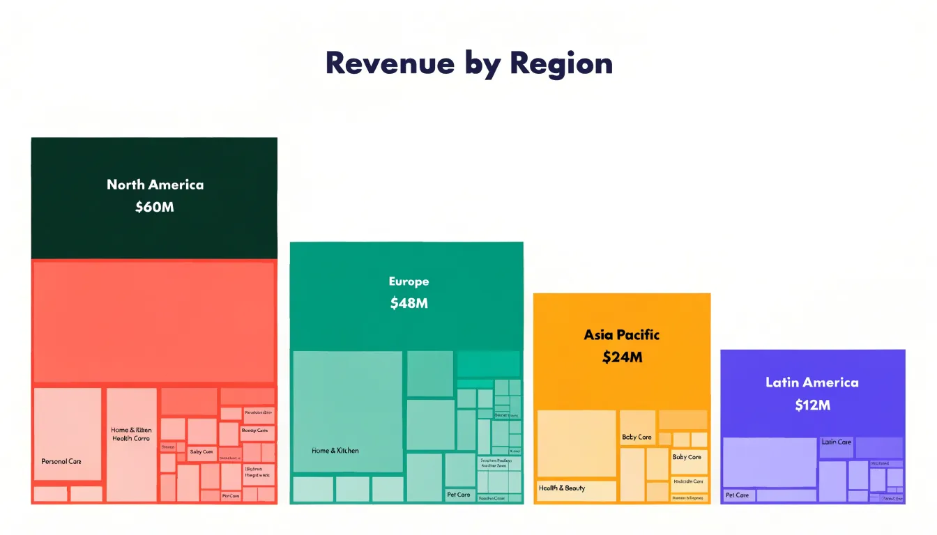
Treemaps offer a powerful way to visualize hierarchical data by nesting rectangles within rectangles, where each rectangle’s area corresponds to a quantitative value. This approach is particularly effective for displaying complex tree-structured datasets, such as organizational budgets, product category sales, or file system storage. By organizing data into nested rectangles, treemaps allow viewers to quickly grasp the relative sizes of different categories and subcategories. The hierarchical structure is preserved through the nesting, so you can see both the big picture—like total revenue by region—and the details—such as individual product contributions within each region.
Color can be used to encode an additional variable, such as profit margin or growth rate, adding another layer of insight. When designing treemaps for presentations, keep the color palette limited and consistent to avoid visual clutter; use contrasting colors for top-level categories and subtle variations for subcategories. Ensure labels are legible by placing them within larger rectangles and using tooltips or callouts for smaller ones. Avoid nesting too many levels, as the smallest rectangles become hard to interpret. Treemaps are ideal for highlighting proportions and patterns across multiple levels, making them a valuable tool for data-driven storytelling in presentations.
Color and Typography
Color and typography are the foundation of chart readability, directly influencing how quickly an audience grasps your key insights. Start with a high-contrast color palette that separates data points, labels, and backgrounds clearly. Use dark text on light backgrounds or vice versa, ensuring a contrast ratio of at least 4.5:1 for normal text and 3:1 for large text. Avoid low-contrast combinations like light gray on white or yellow on white, which force squinting and distract from the message. For data series, choose colors that are distinct in both hue and lightness so they remain distinguishable even for audience members with color vision deficiencies. Tools like ColorBrewer or contrast checkers can help validate your palette.
Typography plays an equally critical role. Establish a clear font hierarchy that guides the eye from the most important element to supporting details. Use a bold, larger font for the chart title and key data labels, a medium weight for axis labels, and a lighter, smaller font for annotations or source notes. Limit yourself to two font families—one for headings and one for body text—to maintain consistency and reduce visual noise. Sans-serif fonts like Arial, Helvetica, or Roboto are generally more legible on screens and projectors. Ensure font sizes are large enough to be read from the back of the room; for presentations, use a minimum of 18-20 points for axis labels and 24-28 points for titles. Avoid decorative fonts, excessive bolding, or all-caps text, which can hinder quick comprehension.
By combining high-contrast colors with a deliberate typographic hierarchy, you direct the audience’s focus to the critical data insights. Every element should serve a purpose; remove or de-emphasize anything that doesn’t. This approach reduces cognitive load, allowing viewers to absorb the information swiftly and make decisions based on the data rather than struggling to decipher the visual.
Data Labels and Layout
Every element on a chart competes for the audience’s attention. Gridlines, legends, and borders are meant to guide interpretation, yet when used excessively they become chart junk that slows comprehension. The goal is to strip away anything that does not directly help the viewer grasp the data.
Start with gridlines: thin, light gray lines can aid reading, but heavy or numerous gridlines create visual noise. Consider removing vertical gridlines entirely and using only a few horizontal ones, or replacing gridlines with direct data labels on the data points themselves. This approach eliminates the need for the viewer to trace back to an axis. Legends often duplicate information that could be placed directly on the chart. When possible, label lines, bars, or pie slices directly, using color and proximity to associate labels with data and remove the back-and-forth eye movement between legend and chart.
Borders and backgrounds add another layer of clutter. A thick border around the chart area or a dark background can distract from the data. Use white space instead of borders to separate the chart from surrounding content. Remove the chart’s outer border and background fill, allowing the data to stand out. Axis lines can also be lightened or removed, with tick marks shortened or eliminated.
The principle is to maximize the data-ink ratio: the proportion of ink used to present actual data versus ink used for non-data elements. A clean chart with aligned labels, a muted color palette, and sufficient background contrast feels open and invites the eye to the key patterns.
Accessibility
Color vision deficiency affects a meaningful share of any audience, with red-green confusion being the most common form. When a chart relies on color alone to separate categories or signal meaning, a portion of viewers may see a muddled picture where distinctions collapse entirely. Building colorblind-friendly visuals starts with palette selection. Tools such as ColorBrewer offer palettes tested for perceptual uniformity, and the widely used Okabe-Ito set provides hues that remain distinguishable for most forms of color blindness. Avoiding red-green pairings for contrast and favoring combinations like blue and orange reduces the risk of confusion. It also helps to vary lightness as well as hue, since luminance differences survive almost every form of color vision deficiency and give each series a distinct visual weight.
Patterns add a second encoding channel that works independently of color. Dashed lines, dotted markers, diagonal hatching, and solid fills let viewers track individual series even when hues appear similar. Pairing every color with a shape, texture, or line style means the chart still reads correctly in grayscale, on a projector with washed-out colors, or in a printed handout. Strong luminance contrast matters for a related reason: light text on a light background or two mid-tone series placed side by side can become hard to separate. Choosing clearly separated lightness values for adjacent elements keeps boundaries crisp for everyone, including viewers with low vision or those watching from the back of a room.
Accessibility checks are straightforward to build into the design process. Previewing a chart in grayscale simulates the loss of hue information and reveals whether the remaining distinctions hold up. Testing with an online color blindness simulator offers a closer approximation of specific deficiencies. These small habits cost little time and keep presentation visuals inclusive and universally intelligible, so every viewer can follow the story the data tells.
Dashboards
A well-crafted dashboard transforms a collection of individual charts into a single, cohesive story. The key is to select chart types that complement one another, each serving a distinct purpose while contributing to the overall narrative. Start with a clear focal point—typically a large, high-level metric or trend that anchors the viewer’s attention. Surround it with smaller, supporting visuals that provide context, such as a breakdown by category or a comparison over time.
Use consistent color schemes and typography to unify the elements, and maintain a logical layout that guides the eye from the most important information to the finer details. Avoid the temptation to include every available data point; instead, prioritize clarity by removing non-essential elements like gridlines, redundant labels, or decorative graphics. White space is your ally—it prevents the dashboard from feeling crowded and allows each chart to breathe. Group related charts together and use subtle dividers or background shading to delineate sections without adding visual noise.
Test the dashboard by asking whether a viewer can grasp the main message within seconds. If not, simplify further. Remember that a dashboard is not a data dump; it is a curated experience designed to inform and persuade. By carefully arranging complementary chart types, you create a unified narrative that resonates with your audience and drives decision-making.
Frequently Asked Questions
When should I use a horizontal bar chart instead of a vertical one?
Horizontal bar charts work well when category names are long, when there are many categories, or when labels would crowd the axis. Vertical bar charts suit a small number of categories with short labels and a natural left-to-right flow.
What is the difference between a stacked bar chart and a 100% stacked bar chart?
Plain stacked bars show the total length as the absolute figure and the colored segments as relative shares, while 100% stacked bars normalize every bar to the same length and emphasize composition instead of absolute comparison. Use plain stacked bars when totals differ and those differences carry meaning, and use 100% stacked bars when the story is about share.
How many lines should I put on a line graph for a presentation?
Limit the number of lines on a single chart to three to five series, which is usually the practical ceiling before the plot becomes a tangle. Differentiate multiple series with distinct colors and direct labels placed near the end of each line.
How many slices should a pie chart have?
Limit a pie chart to about five slices to keep it legible and prevent visual clutter. If there are more categories, group the smallest values into a single “Other” slice, and use a bar chart when values are nearly identical because close comparisons are difficult to distinguish in a circle.
What should I watch out for when designing a gauge chart?
Gauges display one value at a time, so they suit a slide that makes a single point rather than a dashboard full of competing dials. Define colored threshold zones before the chart is drawn, keep the arc short typically as a half-circle, and make sure colored zones remain distinguishable for colorblind viewers through labels or pattern cues.
What contrast ratio should I use for chart text and labels?
Use a contrast ratio of at least 4.5:1 for normal text and 3:1 for large text. Use dark text on light backgrounds or vice versa, and avoid low-contrast combinations like light gray on white or yellow on white.
Tony Astor
Tony writes about data visualization and the tools people use to build charts and dashboards. More about Data Illustrator