Best Charts for Marketing Data and Campaign Results
 By Tony Astor ·

Best Charts for Marketing Data and Campaign Results
Bar charts are the default for comparing campaign results across channels, while line graphs track metrics over time, funnel charts show stage-by-stage drop-off, and pie charts display audience splits. Other options include area charts for cumulative reach, scatter plots for correlations, heat maps for page behavior, cohort charts for retention, and Sankey diagrams for multi-touch journeys.
Table of Contents
Bar Charts
Bar charts are a dependable tool for comparing campaign results across channels because they map directly onto how marketing data is structured. Campaign performance usually arrives as discrete categories—Facebook, Google Ads, email, organic search, display—each producing measurable outcomes such as clicks, conversions, cost per acquisition (CPA), and return on investment (ROI). A bar chart represents each channel as a separate bar whose length or height corresponds to the metric’s value. When a marketing manager presents a chart where the bar for email towers over the bar for display advertising on conversions, leadership grasps the gap in seconds.
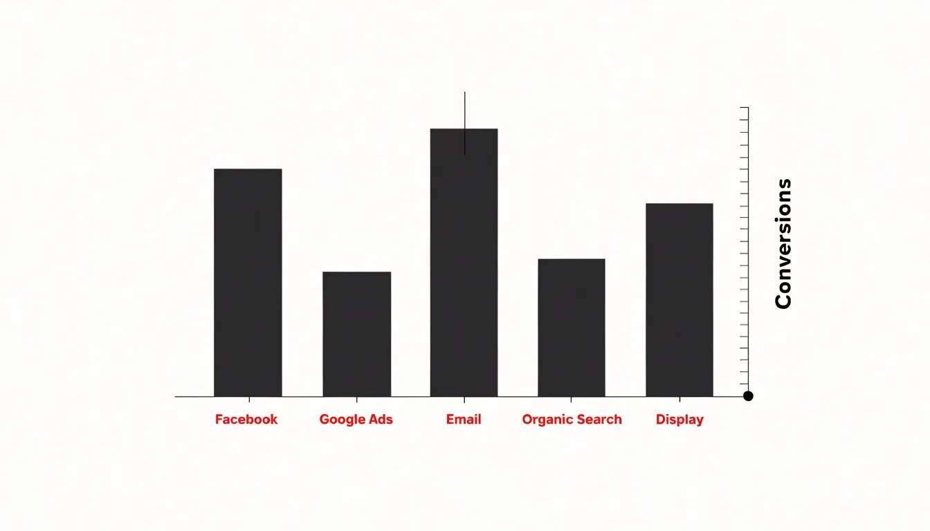
Because all bars share a baseline and scale, viewers can judge relative performance more accurately than they can with charts based on area or angle. Marketers can group bars to show multiple metrics side by side for each channel (such as clicks and conversions), or use separate charts when units differ, such as spend in dollars versus conversion counts. Horizontal bars work especially well when channel names are long, since the labels sit comfortably along the vertical axis.
Bar charts also handle period-over-period comparisons cleanly. A grouped bar chart can pit this quarter against last quarter for every channel, while a stacked bar chart breaks total conversions down by channel within each period. This flexibility makes the bar chart a practical default for channel comparison.
Line Graphs
Line graphs track how a metric moves across a continuous span, making them the natural choice for data that unfolds over days, weeks, months, or quarters. Plotting time on the horizontal axis and a measured value on the vertical axis, a line graph connects each data point in sequence to reveal trajectory: whether website traffic is climbing steadily, dipping on weekends, or flattening after a campaign launch. Flat tables of daily numbers obscure this shape of change.
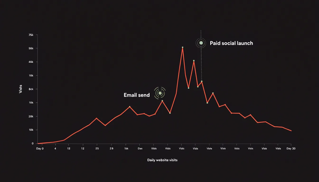
Plotting daily visits over a month immediately shows which days spike after an email send or paid social push and which days trail off. Weekly lead generation works the same way, showing whether the pipeline is accelerating or losing momentum before an important sales cycle. For monthly recurring revenue, a rising line signals healthy retention and expansion, while a declining line points to churn that warrants attention.
Multiple lines, each with a distinct color and clear legend, let you track channels such as organic search, paid ads, and email referrals over the same period. Annotations marking launches, pricing changes, or holidays add context to spikes and dips. To keep the chart readable, limit the number of lines, label axes clearly, choose time intervals that match your reporting cadence, and set a scale that does not exaggerate minor fluctuations.
Funnel Charts
Funnel charts map the customer journey from first impression to final purchase as a series of progressively narrower horizontal segments. Each segment represents a distinct phase—such as awareness, interest, consideration, intent, and conversion—and its width corresponds to the number of remaining prospects, immediately showing where volume is lost.
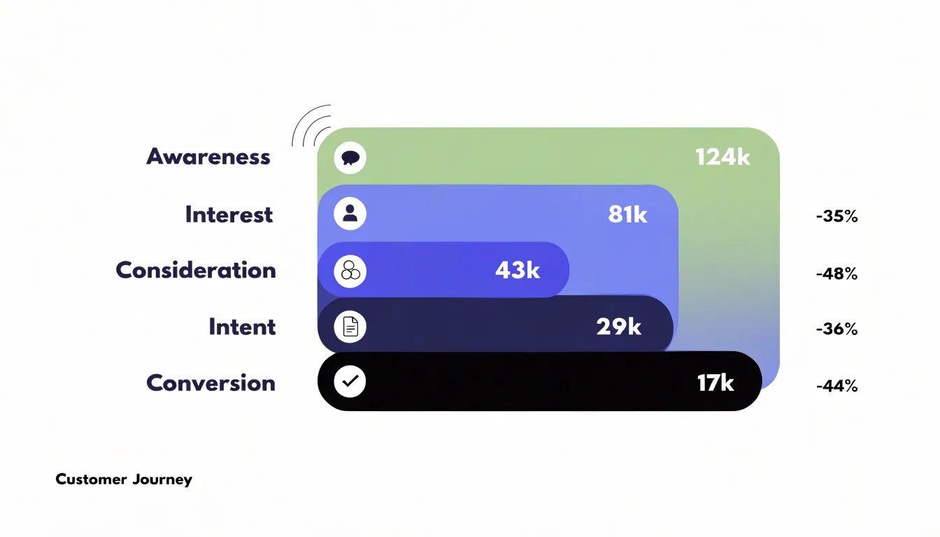
By comparing the number of people who enter a stage with the number who progress to the next, marketers can calculate drop-off rates that pinpoint where prospects abandon the journey. A steep narrowing between consideration and intent tells a team that messaging, pricing, or product presentation is deterring interested prospects. A gentler slope between awareness and interest suggests top-of-funnel content is capturing attention effectively.
Rather than tracking raw numbers in isolation, teams can use this stage-by-stage view to diagnose conversion bottlenecks and prioritize optimization where the largest gaps appear. Marketers can also compare performance across channels, time periods, or audience segments by placing multiple funnels side by side. When a campaign underperforms, the funnel shape reveals whether the problem sits at the entry point, in the middle of the journey, or at the final conversion step.
Pie Charts
Pie charts show how a whole audience divides into segments, suiting demographic breakdowns, traffic source splits, and customer segment percentages. To keep them readable, follow a few rules:
- Limit slices to five or six. Group smaller categories into an “Other” slice, and ensure each slice represents a meaningful share—typically at least 5%.
- Order slices from largest to smallest. Start at the 12 o’clock position and move clockwise so readers can quickly grasp relative sizes.
- Label directly. Put the category name and percentage on each slice to spare readers from consulting a legend, and use distinct, high-contrast colors from your brand palette. Add a small companion table if precise values matter.
- Skip visual clutter. Avoid 3D effects and exploded slices, which distort proportions, as well as unnecessary gridlines, borders, and background images.
If your data includes negative values or parts that do not sum to a meaningful whole, choose a bar chart instead. For audience breakdowns with many categories, a bar chart or treemap is usually more effective. Use pie charts sparingly—perhaps one per dashboard—to maintain their impact.
Area Charts
Area charts visualize cumulative growth and total reach over time by filling the space beneath a line with color. They make it easy to see whether overall brand reach is expanding steadily, plateauing, or accelerating during a particular phase of a campaign.
Their distinct strength is layering multiple series on the same timeline. Each channel appears as a colored band stacked so the combined height reflects total reach while individual bands show each channel’s contribution. A team can see, for example, that organic search drives consistent baseline growth while paid social contributes a burst of reach during a product launch.
This dual view serves two audiences at once. Stakeholders who need a high-level picture of brand reach can look at the top edge of the chart, while channel owners can examine the thickness of their own band over time. Shifts in a channel’s contribution appear as changes in the stack’s proportions, eliminating the need for separate charts for each source.
Scatter Plots
A scatter plot answers whether two metrics move together. Each point represents a single unit—one campaign, one ad set, or one day of spend—placed according to its values on two axes. Plotting cost-per-click on one axis and engagement rate on the other reveals the relationship’s shape. A tight cluster rising from left to right suggests higher click costs accompany higher engagement, while a downward drift points to an inverse relationship. A wide, formless scatter indicates the two variables have little to do with each other, which is itself useful when deciding which levers to pull.
Points that break away from the main group are especially telling. These outliers represent campaigns that delivered engagement far above or below what their click costs would predict. A point sitting high on the engagement axis with low cost-per-click marks a campaign whose creative, audience, or placement choices may be worth replicating. Points sitting low despite heavy spend often expose wasted budget or targeting mismatches. Coloring points by channel or adding a trend line makes these patterns easier to read when deciding where to shift resources for the next flight.
Heat Maps
Heat maps provide a visual record of how visitors behave on a landing page. Rather than relying on aggregate metrics, a heat map overlays color directly onto the page, using warmer tones for heavy activity and cooler tones for overlooked areas. It captures three main behavioral signals:
- Click density: Highlighting where visitors click most often shows which buttons, links, and calls to action attract genuine interest. It also exposes design mismatches, such as visitors repeatedly clicking an image or headline that looks interactive but is not.
- Scroll depth: Tracking how far down the page visitors travel segments behavior into engagement bands. Sections most visitors never reach can be repositioned, condensed, or cut, while content that consistently draws scrolling can be given prime placement.
- Interaction cold spots: Areas with little clicking or scrolling often signal weak headlines, confusing layout, or visual clutter that pushes attention away.
Together, these three lenses guide concrete UX tests—simplifying layouts, moving key offers into view, and removing distractions—to lift conversion on campaign landing pages.
Stacked Bar Charts
Stacked bar charts let marketers read two layers of information at once: the full height of each bar shows a total figure (such as total channel traffic or campaign conversions), while the segments inside divide that total into its component parts. A single visual can show that email drove the most site visits in a quarter while also revealing how much of that volume came from organic newsletter sign-ups versus paid sponsored placements. Viewers compare channels horizontally across bars and sub-metrics vertically within each bar.
This structure helps when a headline number hides an important compositional shift. A stacked bar chart of organic versus paid traffic might reveal that a channel’s total volume looks stable only because paid placements are quietly expanding as organic share shrinks—a trend a standard bar chart would collapse into one figure.
Stacked bars also work well for breaking each channel down by new versus returning visitors, or desktop versus mobile sessions. Keep the number of segments small and order them consistently across bars so viewers can compare proportions without effort.
Treemaps
Treemaps represent hierarchical data as nested rectangles whose sizes are proportional to a value such as spend or revenue. For marketing budgets, the largest rectangle represents total spend, subdividing into departments, then campaigns within each department, and finally individual tools or channels. This nested structure mirrors how budgets cascade through an organization, showing which areas consume the most resources and how smaller line items roll up.
Color adds a second dimension, flagging metrics like return on ad spend (ROAS), CPA, or variance against plan so a single view communicates both allocation and performance. Because rectangles scale to fill available space, treemaps handle dozens or hundreds of line items more compactly than spreadsheets. Leaders can quickly spot an oversized block for a low-performing channel or a cluster of small tool subscriptions that add up to a significant share of spend, and can answer questions about a specific campaign by pointing directly to its rectangle within a department block.
When building a treemap, keep categories consistent, group tiny items into an “Other” block, and label the largest rectangles directly.
Waterfall Charts
Waterfall charts show how individual campaigns build toward net revenue by stepping through positive and negative financial impacts in sequence. Each bar represents a single campaign or initiative, moving from left to right. Positive contributions rise above the previous level, while negative impacts—such as campaign costs or underperforming initiatives—drop below it, tracing how each activity contributes to the final total rather than presenting that total as an unexplained figure.
When presenting results to stakeholders, a waterfall chart makes the link between spend and return explicit. A profitable campaign appears as an upward step and a money-losing campaign as a downward step, helping justify budget shifts for future planning.
Bar ordering shapes the narrative. Teams often group positive returns together before showing costs and deductions, or sequence campaigns chronologically to match the marketing calendar. Color coding reinforces the distinction between gains and losses. Waterfall charts remain legible when limited to roughly a handful to a dozen campaigns.
Gauge Charts
Gauge charts use a needle or filled arc moving across a defined scale toward a marked target to show where a single metric stands against a threshold. In marketing reports, this suits KPIs with a clear goal or ceiling, such as a quarterly lead-generation target, a customer acquisition cost limit, or a target ROAS. Built-in color bands reinforce the reading: green for healthy progress, amber for a softening trend, and red for a shortfall.
This immediacy makes gauges popular on executive dashboards, where senior stakeholders want a quick status check before drilling into channel-level data. A row of gauges, each tied to a distinct quarterly objective, provides a consolidated health check in seconds.
Dedicate each dial to a single metric with a known target and a sensible scale. Pairing the gauge with a small numerical readout of the current value and the percentage of the goal attained keeps the display precise without adding clutter.
Cohort Charts
Cohort charts track how distinct groups of customers behave after acquisition. A cohort is defined by a shared starting point—such as the month a customer made a first purchase, signed up for a trial, or responded to a campaign. The chart lists these groups as rows and plots subsequent time periods (usually weeks or months) across the columns. Each cell shows the percentage or count of that original group that returned, purchased again, or remained active during that period.
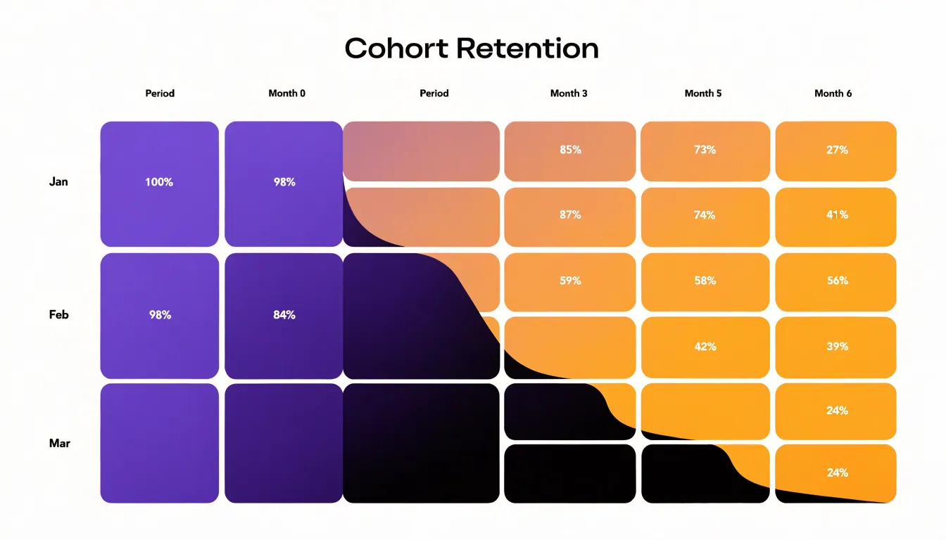
Reading across a row reveals a cohort’s retention curve: a steep drop in early columns shows rapid disengagement after acquisition, while a flatter slope signals lasting engagement. Comparing rows shows whether newer cohorts retain better or worse than older ones, helping teams judge whether recent changes to onboarding, messaging, or product experience are working. Overlaying revenue per cohort turns the grid into a lifetime value view, highlighting which acquisition periods produced customers who kept spending over many months.
By separating acquisition timing from post-acquisition behavior, cohort grids preserve variations that a single average retention rate would hide. Marketers can spot seasonal effects, evaluate lead quality by channel, connect campaigns to long-term outcomes, and use mature cohorts’ retention curves to forecast the value of newly acquired customers.
Sankey Diagrams
Sankey diagrams visualize how users move through multi-touch marketing funnels where journeys branch across several channels and pages. Connected bands represent paths, with each band’s width proportional to the volume of users traveling along it.
A marketing Sankey diagram typically starts with traffic sources (organic search, paid social, email, direct visits) on the left, flows through intermediate touchpoints (landing pages, product pages, sign-up forms) in the middle, and ends at conversion events (purchases, newsletter sign-ups, demo requests) on the right. Because band width reflects user volume, dominant routes and thin, underperforming branches stand out immediately.
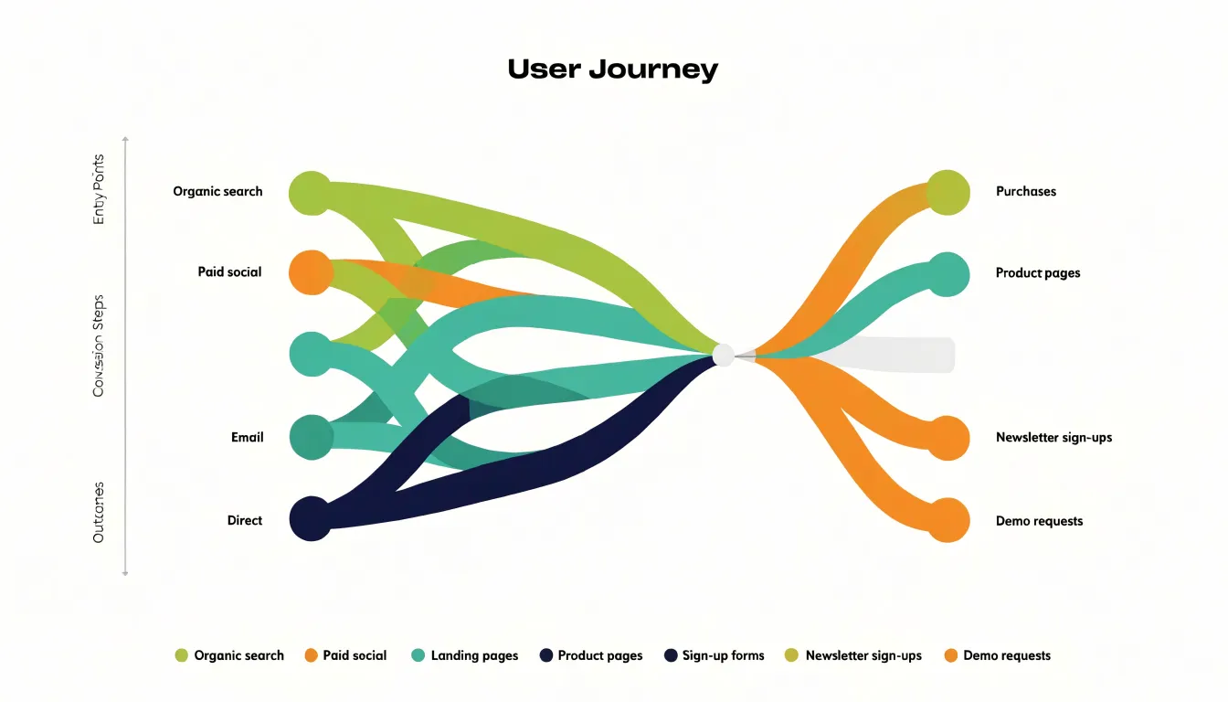
Real customer journeys rarely follow a single straight line, and Sankey diagrams accommodate that non-linear behavior by displaying multiple simultaneous routes in one connected view. Teams can see which sources feed the most valuable downstream outcomes and which pages act as bottlenecks where volume narrows sharply, informing decisions about multi-touch attribution, budget allocation, and page optimization.
Dashboard Layouts
When several charts share a screen, their arrangement shapes how stakeholders read the data. A clear dashboard layout moves from broad summary to fine detail in three bands:
- Top band (Executive summary): Place a small set of headline metrics or a single overall trend line at the top to answer whether performance is on track before viewers invest attention in detail.
- Middle band (Diagnostic breakdowns): Use the center for campaign-by-campaign comparisons, channel breakdowns, and segment performance that explain movements in the headline figures.
- Bottom band (Granular detail): Reserve the bottom for individual ad sets, creative variations, geographic splits, or daily pacing—the data that answers where to take specific action. Positioning the finest detail last matches how readers naturally move from scanning to investigating and keeps the screen from overwhelming casual viewers.
Maintain uniform color coding, aligned time frames, and consistent axes across all three bands so a stakeholder can trace a dip in the top-line trend directly to the channel and ad set responsible. Brief annotations on key metrics provide the context needed to connect the charts into a coherent report.
Frequently Asked Questions
What is the best chart for comparing campaign results across channels?
Bar charts are a dependable choice for comparing campaign results across channels because they map discrete categories like Facebook, Google Ads, and email to separate bars on a shared baseline and scale. They can also show multiple metrics side by side or compare periods.
How can I track a marketing metric over time?
Line graphs track how a metric moves across a continuous span such as days, weeks, months, or quarters. Multiple lines with a clear legend can compare channels like organic search, paid ads, and email referrals over the same period.
What does a funnel chart show in marketing?
Funnel charts map the customer journey from first impression to final purchase as progressively narrower segments. Comparing who enters each stage with who progresses to the next helps calculate drop-off rates and pinpoint conversion bottlenecks.
When should I avoid using a pie chart?
Avoid pie charts if the data includes negative values or parts that do not sum to a meaningful whole, and choose a bar chart instead. For audience breakdowns with many categories, a bar chart or treemap is usually more effective.
What can a heat map tell me about a landing page?
Heat maps show click density, scroll depth, and interaction cold spots on a landing page. These signals can guide UX tests such as simplifying layouts, moving key offers into view, and removing distractions.
How should charts be arranged on a marketing dashboard?
A clear dashboard layout moves from broad summary to fine detail: headline metrics at the top, diagnostic breakdowns in the middle, and granular detail at the bottom. Uniform color coding, aligned time frames, and consistent axes help stakeholders trace top-line changes to the responsible channel or ad set.
Tony Astor
Tony writes about data visualization and the tools people use to build charts and dashboards. More about Data Illustrator