Best Charts for Financial Data
 By Tony Astor ·
Best Charts for Financial Data
Line graphs track continuous price trends and moving averages, candlestick charts compactly show open, high, low, and close prices to reveal market sentiment, and bar charts compare discrete categories like departmental revenue. Waterfall, area, scatter, bubble, treemap, heat map, histogram, combo, bullet, sparkline, and gauge charts each suit specific financial tasks.
Table of Contents
Line Graphs
Line graphs serve as the foundational tool for tracking stock trends because they represent price data as a continuous flow rather than as isolated events. Each point on the line corresponds to a specific closing price at a given moment, and connecting those points shows how a security has moved through time. This continuous representation makes it easy to spot the overall direction of a stock, whether it is climbing steadily, drifting sideways, or descending through a prolonged downturn. Because the eye naturally follows the connected path, investors can quickly grasp the rhythm of price movement without parsing dense tables of numbers.
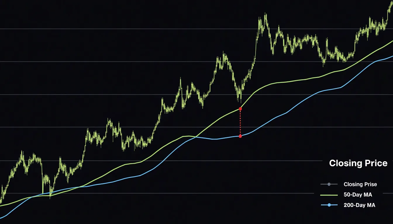
Moving averages become far more interpretable when plotted directly onto a line graph. A simple moving average smooths out short-term volatility by calculating the mean price across a rolling window, and overlaying this smoother line on the raw price series reveals the underlying trajectory. Where the price line crosses above or below its moving average, analysts often read signals about momentum shifts. Longer moving averages, such as the 200-day line, help distinguish temporary fluctuations from genuine changes in trend direction.
Long-term equity growth is another strength of the line graph format. By extending the horizontal axis across months, years, or decades, a single chart can capture the compounding effect of sustained appreciation alongside periodic corrections. Investors can compare the slope of growth during bull markets with the flattening that occurs during recessions, gaining perspective on how a holding has performed through complete market cycles.
Customizable timeframes add flexibility to the format. A viewer can zoom from an intraday view showing hourly fluctuations to a multi-year perspective showing broad secular trends, all within the same visual language. This adaptability makes line graphs equally useful for day traders monitoring short-term movements and for long-term investors evaluating whether a stock aligns with their portfolio horizon.
Candlestick Charts
Candlestick charts are a cornerstone of financial technical analysis, offering a compact visual summary of price action over a given period. Each candlestick represents four key data points: the open, high, low, and close (OHLC) prices. The body of the candle, formed by the open and close, indicates the direction of price movement: a green or white body signifies a bullish session where the close exceeds the open, while a red or black body denotes a bearish session where the close falls below the open. The thin lines extending from the body, known as wicks or shadows, mark the high and low prices reached during the period, providing insight into intraday volatility and the range of trading activity.
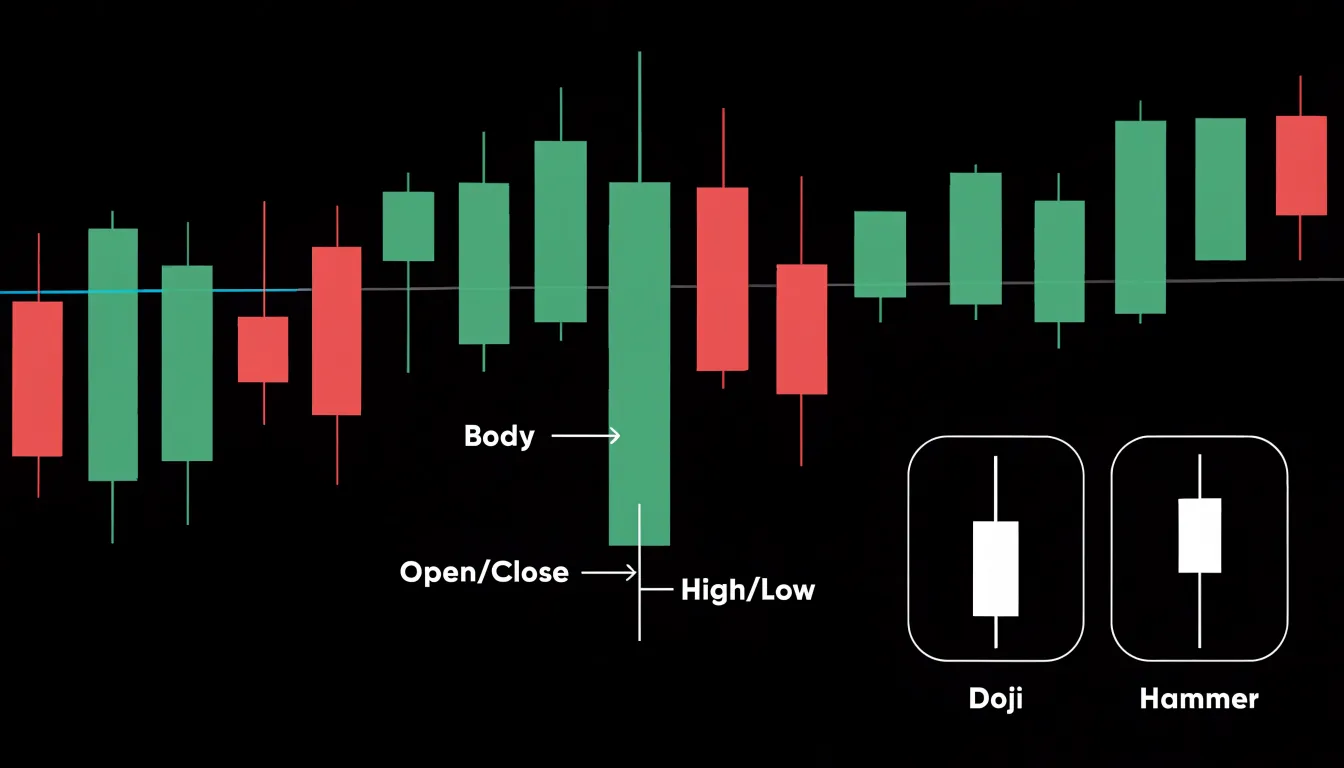
The relationship between these OHLC values reveals market sentiment and potential turning points. For instance, a long lower wick suggests that sellers drove prices down but buyers stepped in to push the close higher, indicating bullish rejection of lower levels. Conversely, a long upper wick hints at bearish pressure near the highs. Candlestick patterns, such as doji, engulfing, and hammer formations, are built on these OHLC dynamics and are widely used to anticipate reversals or continuations. The size of the candle body relative to its wicks also conveys volatility: a large body with short wicks indicates strong directional momentum, while a small body with long wicks signals indecision and heightened intraday fluctuation. By analyzing candlestick charts, traders can gauge the balance of power between buyers and sellers and identify emerging trends in fast-moving financial markets.
Bar Charts
Bar charts excel at comparing discrete categories, making them a natural fit for financial data such as revenue across departments. Each department—sales, marketing, operations, finance—is represented by a separate bar, and the length of each bar corresponds to its revenue figure. This direct visual encoding allows viewers to instantly see which business units are top performers. If the sales department consistently generates the highest revenue, its bar will tower over the others, providing an immediate sense of relative performance on executive dashboards.
Beyond simple rankings, bar charts are effective for highlighting quarterly sales variance. By grouping bars by quarter (e.g., Q1, Q2, Q3, Q4) and coloring them by department, or by using clustered bar charts, you can compare how each department’s revenue fluctuates over time. This makes it easy to spot seasonal trends, identify departments that are meeting targets, and flag those that are underperforming. For example, a department that consistently falls short in Q4 might indicate a need for strategic adjustments.
Bar charts also facilitate cross-departmental earnings comparisons. When multiple departments are displayed side by side, stakeholders can quickly assess which units contribute most to overall profitability and which may require investment or restructuring. Sorting bars by value further enhances this analysis, allowing for immediate identification of leaders and laggards.
Waterfall Charts
A waterfall chart is a specialized form of bar chart that displays how an initial value is affected by a series of intermediate positive and negative changes, culminating in a final result. In financial reporting, this structure makes it an ideal tool for presenting a profit and loss statement as a visual bridge from gross revenue down to net income. Each bar in the chart represents a single line item, such as cost of goods sold, operating expenses, or taxes, and each bar floats from the cumulative total of the preceding items, so the reader can follow the step-by-step progression with a single glance.
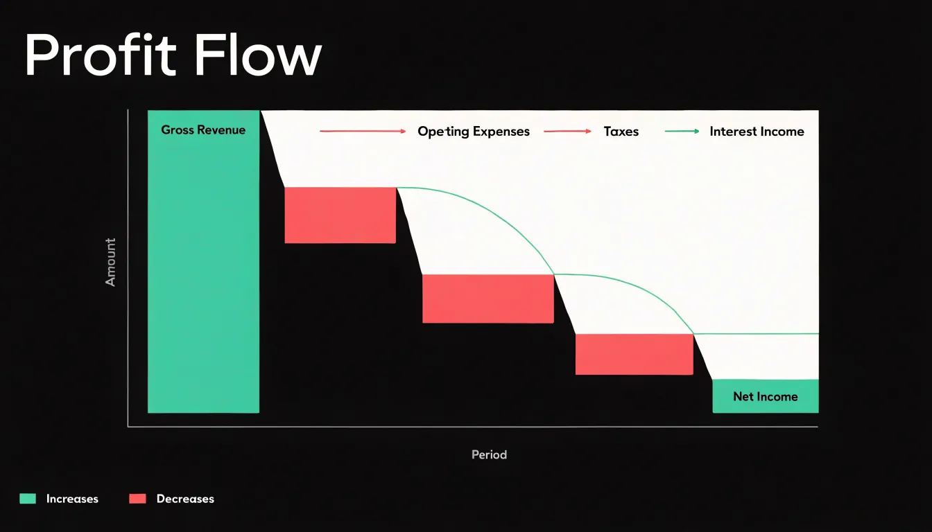
The first bar typically shows gross revenue as a full column rising from the baseline. Subsequent bars representing deductions, such as cost of goods sold, appear as downward steps that begin at the top of the revenue bar and descend to a new cumulative level, giving a visual shape that mirrors the arithmetic of the statement. Items that add to income, such as interest income or gains on asset sales, appear as upward steps that lift the running total. Subtotals such as gross profit or operating income can be rendered as solid columns resting on the baseline, which helps readers pause at key checkpoints along the journey.
Color coding reinforces the meaning of each step, with increases and decreases rendered in distinct hues so that the direction of each contribution is immediately legible. Connector lines between the bars guide the eye along the cumulative path, and data labels placed at each step allow precise values to be read without cluttering the layout. The descending staircase from gross revenue to net income gives viewers an intuitive sense of where margin is gained or lost, showing at a glance which cost categories consume the largest share of revenue. Because the chart preserves the sequential logic of the profit and loss statement, it supports both executive summaries and detailed variance analysis, making the path from top-line revenue to bottom-line earnings visible as a coherent progression rather than a list of isolated figures.
Area Charts
Area charts map cumulative financial growth by filling the space beneath a line with a solid or gradient shade, turning a trend into a visual representation of total volume. The shaded region under the curve emphasizes the magnitude of accumulation, making it easy to see how values build over time. When tracking a portfolio’s value, an area chart displays the rising total as a growing block of color, so the aggregate capital buildup is immediately apparent even across decades.
Stacked area charts extend this concept by layering multiple data series on top of one another, with each band’s height representing its contribution to the whole. This stacking technique is particularly effective for visualizing the composition of a portfolio as it evolves: individual holdings or asset classes appear as distinct colored bands, and the overall height of the stack shows the combined value. Investors can quickly discern which components drive growth and how the mix shifts over extended periods.
The continuous shaded area highlights the cumulative nature of financial growth, where each period’s gains add to the previous total. This makes area charts ideal for illustrating long-term trends such as retirement savings, where regular contributions and compounding returns create an ever-widening area under the curve. By focusing on the total area rather than just the line, viewers grasp the scale of capital buildup and the sustained impact of incremental growth.
Scatter Plots
A scatter plot places one variable on each axis, and in financial analysis a common pairing is volatility on the horizontal axis against expected return on the vertical axis. Each asset, fund, or strategy appears as a single point, positioned according to its measured risk and its anticipated yield. This arrangement shows where each opportunity sits relative to the risk it demands and how those positions cluster together. When points form a pattern rising from lower-left to upper-right, the chart shows the familiar tradeoff in which higher expected returns accompany higher volatility. When points spread widely at the same level of risk, the plot reveals dispersion in risk-adjusted performance, flagging assets whose returns lag or lead their peers even though they carry comparable uncertainty.
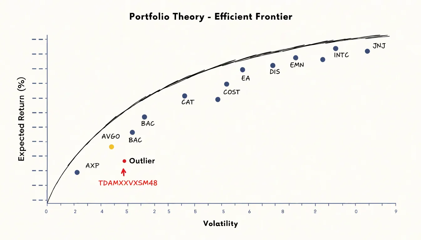
The efficiency of a diversified portfolio becomes easier to examine through this lens. Assets that fall below the general trend line deliver less return than their volatility would suggest, while those above it reward each unit of risk more generously. By sketching the boundary formed by the most favorable combinations, analysts can see the efficient frontier taking shape and judge whether their current holdings sit near it or drift toward inefficiency. Outliers deserve particular attention: a point far from the main cloud may signal a genuinely superior risk-adjusted performer, an asset mispriced by the market, or a data anomaly worth verifying before any decision is made.
Stakeholders can absorb this risk-return landscape at a glance and compare individual positions against benchmarks and peer groups. Careful labeling, consistent scaling, and clear annotations of outliers keep the chart readable and prevent misleading impressions, making the scatter plot a practical instrument for portfolio review and diversification analysis.
Bubble Charts
Bubble charts extend the scatter plot by introducing a third dimension through the size of each data point. In financial analysis, this allows for the simultaneous comparison of market capitalization, return on investment, and relative trading volume within a single visual framework. Each bubble represents an individual asset, with its position on the x and y axes corresponding to two key metrics, such as market cap and return, while the bubble’s size encodes a third metric, like trading volume.
This multi-dimensional approach enables analysts to quickly identify patterns and outliers that might be missed when examining metrics in isolation. For instance, a large bubble positioned in the upper-right quadrant indicates a company with high market valuation, strong returns, and significant trading activity, often a market leader. Conversely, a small bubble in the lower-left quadrant suggests a smaller, underperforming asset with low liquidity. The visual clustering of bubbles can reveal sector trends or market segments, while the size variation helps assess liquidity and investor interest.
Bubble charts are particularly useful for portfolio diversification analysis, as they highlight the relationship between risk (often represented by market cap or volatility) and reward (returns), with volume providing context on market sentiment. However, effective use requires careful scaling of bubble sizes to avoid misinterpretation, as area perception is less precise than position.
Treemaps
Treemaps translate hierarchical market structures into nested rectangles, where the entire canvas represents the whole market and each subdivision carves out space proportional to its share. At the top level, broad market sectors occupy large blocks of the display, so the technology, healthcare, or energy sectors each claim a portion of the canvas that mirrors their aggregate weight in the index or portfolio. Within each sector block, individual companies appear as smaller rectangles sized by market capitalization, creating a visual hierarchy that moves from the widest category down to the single stock. This nesting allows investors to see sector weightings and relative asset capitalization in one glance, without switching between separate tables or pie charts.
The area of every rectangle corresponds directly to a quantitative value, so a company twice the size of its neighbor occupies twice the space. Color adds a second dimension: rectangles can be shaded to reflect daily price change, valuation multiples, or dividend yield, so the treemap communicates both structural composition and current performance simultaneously.
Because the layout packs rectangles tightly, treemaps use screen space efficiently even when hundreds of companies are displayed, which suits market overview dashboards and heat maps of index constituents. Analysts can quickly identify where capital concentrates, spot sectors that dominate the benchmark, and recognize small-cap positions that fill the remaining corners of the grid. Squarified treemap algorithms keep rectangles close to square shapes, improving readability of labels and reducing distortion. The result is a compact, hierarchical snapshot of market composition that supports sector allocation decisions and highlights the relative importance of each holding.
Heat Maps
Heat maps translate dense numerical tables into color-coded grids where each cell represents an asset, sector, or metric, and the intensity of the color corresponds to the magnitude of its value. For traders scanning dozens or hundreds of instruments at once, this visual encoding removes the need to read individual numbers, allowing the eye to land immediately on the brightest greens and deepest reds.
In equity markets, a sector heat map arranges companies into blocks sized by market capitalization and shaded by daily percentage change, so an entire portfolio’s exposure can be assessed in a single glance. The same principle extends to valuation shifts: shading cells by price-to-earnings ratio or earnings revisions reveals which segments of the market have become richly priced or have quietly de-rated over a period. Liquidity analysis benefits equally, since bid-ask spreads, order book depth, or trading volume can be mapped across instruments to expose thin markets before a position is opened.
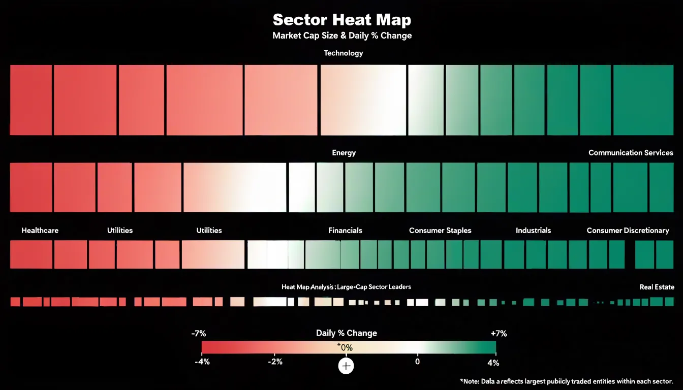
A practical advantage of heat maps is their compactness; a grid of a few hundred cells fits comfortably on one screen and updates in real time, making it a natural dashboard companion to candlestick or line charts that drill into individual names. Traders typically pair a heat map with a click-through workflow, using the map to identify outliers and then opening the underlying security for detailed inspection. The technique works best when color scales are chosen deliberately, with diverging palettes centered on zero for percentage changes and sequential palettes for absolute measures such as volume. By compressing cross-sectional comparisons into a pattern of color, heat maps turn market-wide monitoring into a rapid visual scan rather than a laborious spreadsheet exercise.
Histogram Charts
Histogram charts give analysts a direct view of how returns or yields are distributed across a continuous range by grouping observations into frequency bins. Each bar represents an interval of values, such as daily returns falling between 0.5 percent and 1.0 percent, and the height of that bar counts how many observations landed inside it. This grouping transforms a long series of raw numbers into a shape that can be read at a glance, revealing whether outcomes cluster tightly around a central value or spread widely across extremes.
When the bars form a smooth bell shape, the data approximates a normal distribution, and analysts can lean on standard statistical assumptions about mean and variance. Deviations from that shape carry important information. A histogram with a long right tail shows positive skew, where occasional large gains pull the average upward while most observations sit lower. A long left tail indicates negative skew, with rare severe losses dragging the distribution downward. Recognizing skewness early helps investors avoid relying on averages that misrepresent typical experience.
The tails of a histogram matter most for risk assessment. By examining the outermost bins, analysts estimate tail-risk probabilities, the likelihood of returns falling beyond a chosen threshold such as three standard deviations from the mean. Fat tails, visible as bars that stay taller than a normal curve would predict at the extremes, signal that extreme events occur more often than standard models assume. This insight informs position sizing, stop-loss placement, and stress testing.
Histograms also support comparison across assets. Overlaying distributions for two portfolios shows which carries wider dispersion or heavier downside tails, guiding diversification decisions. Bin width selection affects readability, so analysts often test several groupings to confirm that observed patterns are robust rather than artifacts of arbitrary intervals.
Combo Charts
A combo chart pairs a column or bar series with a line series inside a single plot area, and in financial analysis the most familiar version overlays a price line on a histogram of trading volume. The volume bars are typically drawn from a zero baseline along the primary vertical axis, while the price series floats on a secondary axis scaled to its own range. This dual-axis layout matters because volume is measured in millions of shares while price might move within a range of a few dollars, so putting both on one scale would flatten the price line into a nearly straight line at the top or bottom of the chart. By assigning each series its own axis, both remain readable and the reader can compare their shapes directly.
The practical value appears during high-activity events such as earnings releases, index rebalances, or macro announcements. A sudden burst in volume shows up as a tall cluster of bars, and the price line running across the same horizontal position reveals how the market responded. A volume spike paired with a steep upward move in the price line signals strong buying conviction, while a similar spike accompanying a flat or declining line suggests heavy selling into strength or distribution. Because the two series share a common time axis, the reader can see momentum shifts at the exact moment activity surges rather than inferring them from separate charts.
Design details deserve attention. Labeling both axes with distinct colors that match their series, adding a legend, and keeping gridlines light helps prevent misreading which scale applies to which element. The overlay works best with a modest number of data points and clear event markers or annotations so that viewers know why a particular bar stands taller than its neighbors.
Bullet Graphs
Bullet graphs offer a compact way to display how actual operational spending measures up against a target budget. Developed by data visualization expert Stephen Few, a bullet graph packs multiple layers of information into a single horizontal bar, making it ideal for dashboards that track financial performance across many cost centers or departments at once.
The core of the graph is a primary measure bar showing current actual spending, overlaid on a shaded background that represents predefined threshold bands. These bands typically correspond to qualitative ranges such as good, satisfactory, and poor, allowing viewers to instantly judge where actual spending falls relative to acceptable limits. A vertical marker line indicates the target budget for the period, so any gap between the measure bar and the target is immediately visible as either an overrun or an underspend.
Because the graph is so compact, dozens of them can be stacked vertically in a single view, giving finance teams a rapid overview of budget adherence across an entire organization without requiring separate charts for each line item. The threshold bands can be calibrated to reflect the specific risk tolerances of each budget category, so a marketing expense line may have wider bands than a fixed-cost utility line. Comparative measures can also be added, such as a lighter secondary bar showing the prior period’s spending, which helps viewers assess trends alongside the current variance. By combining actuals, targets, and performance bands in one minimal footprint, bullet graphs support fast assessment of expense variances and keep attention focused on the items that require corrective action.
Sparklines
Sparklines are word-sized line graphs that sit directly inside a table cell, typically alongside a row of numbers. In a financial summary, each row might represent a product line, a regional office, or a portfolio holding, with columns for revenue, cost, and margin. Adding a sparkline column turns each of these rows into a compact visual record of movement over time. A reader scanning the table sees not only the current figure but the shape of how it arrived there — a steady climb, a mid-year dip, a sharp recovery in the final quarter. This inline context arrives without requiring the reader to leave the table, open a separate chart, or mentally reconstruct a trend from a list of monthly values.
The value of sparklines lies in their restraint. A full line chart placed beside a table competes for space and attention, and a grid of even a dozen such charts would overwhelm the page. Sparklines are deliberately minimal: no axes, no gridlines, no labels, often just a single line with an optional marker for the high and low points. Because they occupy roughly the height of a line of text, they integrate into the row rhythm of the table rather than interrupting it. A financial summary can carry twenty or thirty of them and still read as a table, not a dashboard.
This makes sparklines particularly effective for comparison across many entities. When every row shares the same sparkline scale and format, patterns emerge at a glance: which regions show consistent growth, which show volatility, which have flattened. The eye can compare shapes faster than it can compare sequences of numbers. Used this way, sparklines function as a lightweight visual index that directs attention to the rows deserving closer inspection, while the precise figures remain available in the adjacent columns.
Gauge Charts
Gauge charts present a single financial metric as a dial, with a needle or filled arc indicating where the current value sits along a defined scale. The scale is bounded by a minimum and a maximum, and often by threshold markers that represent targets, warning levels, or regulatory limits. This structure makes a gauge chart a natural fit for monitoring executive KPIs that executives review repeatedly, such as net profit margin or the debt-to-equity ratio. In each case, the viewer needs one answer quickly: where does performance stand relative to the goal right now?
When a net profit margin gauge is connected to a live data feed, the needle moves as revenue and costs update, giving leadership a real-time read on profitability without requiring them to interpret a table or recalculate a ratio. Colored zones on the dial can encode interpretation directly. A green band might mark the range at or above target, amber a watch zone, and red a level that demands intervention. A debt-to-equity gauge works the same way, with the scale oriented so that higher leverage pushes the needle toward the risk zone. Executives can absorb the status at a glance and know whether the metric is healthy, drifting, or in breach.
Gauges work best when each one is dedicated to a single measure and placed on a dashboard alongside related indicators. Grouping a profitability gauge with liquidity and leverage gauges gives a compact snapshot of overall financial health. Clear labeling of the target value, the current value, and the units keeps the dial unambiguous, helping decision-makers spot when a metric crosses a threshold and needs attention before it appears in a periodic report.
Dashboard Overview
Financial dashboards integrate multiple chart types—such as line charts for trends, bar charts for period comparisons, and pie charts for composition breakdowns—into a single view. This eliminates the need to toggle between disparate reports.
For board-level reporting, dashboards present key metrics like revenue growth, expense ratios, and cash flow in a consistent format. The layout typically follows a logical hierarchy, starting with high-level summaries and drilling down into granular details so board members can grasp the overall financial position while exploring specific areas of interest.
Unified dashboards also make it easier to spot correlations and anomalies that might be missed when viewing charts in isolation. For instance, a spike in expenses can be immediately cross-referenced with revenue trends, providing context and prompting timely action. Integrating real-time data feeds keeps these insights up to date, creating a single source of truth that reduces misinterpretation and saves time for both preparers and consumers of financial reports.
Frequently Asked Questions
What is the best chart for tracking stock price trends?
Line graphs are a foundational tool for tracking stock trends because they show price data as a continuous flow and make the overall direction of a stock easy to spot. Moving averages can also be plotted on a line graph to help reveal underlying trajectory and momentum shifts.
What do green and red candlesticks mean?
A green or white candlestick body signifies a bullish session where the close exceeds the open, while a red or black body denotes a bearish session where the close falls below the open. The wicks mark the high and low prices reached during the period.
How does a waterfall chart show how gross revenue becomes net income?
A waterfall chart is a specialized bar chart that displays how an initial value is affected by positive and negative changes to reach a final result. In financial reporting, each bar represents a line item such as cost of goods sold, operating expenses, or taxes, creating a visual bridge from gross revenue down to net income.
What are stacked area charts used for?
Stacked area charts layer multiple data series on top of one another, with each band’s height representing its contribution to the whole. They are effective for visualizing how a portfolio’s composition evolves and which holdings or asset classes drive the combined value.
What is the difference between a scatter plot and a bubble chart?
A scatter plot places one variable on each axis, such as volatility against expected return, with each asset shown as a point. A bubble chart extends the scatter plot by using the size of each point to encode a third metric, such as trading volume.
How do traders use heat maps to scan the market?
Heat maps turn dense numerical tables into color-coded grids, where color intensity corresponds to the magnitude of a value. In equity markets, a sector heat map arranges companies into blocks sized by market capitalization and shaded by daily percentage change, allowing a portfolio’s exposure to be assessed in a single glance.
Tony Astor
Tony writes about data visualization and the tools people use to build charts and dashboards. More about Data Illustrator