Best Charts for Demographic Data
 By Tony Astor ·

Best Charts for Demographic Data
Population pyramids are the standard chart for demographic data, using back-to-back horizontal bars to show males and females by age cohort. The silhouette instantly reveals a population’s structure: a broad base signals a youth bulge, a narrow base with wider upper bars indicates an aging population, and symmetry shows balanced cohort sizes.
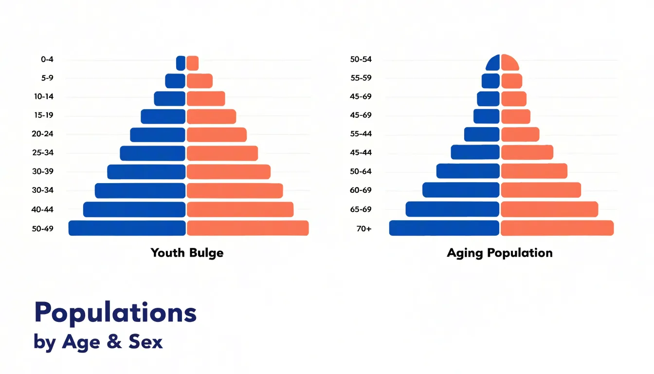
Table of Contents
Population Pyramids
Population pyramids present a dual-axis bar chart in which each horizontal bar represents an age cohort, with males extending to one side and females to the other. This back-to-back layout lets readers compare the size of each age-sex group instantly, tracking the length of bars from the base upward. The shape that emerges carries immediate meaning about a population’s structure: a broad base indicates a youth bulge, where a large share of the population is concentrated in younger cohorts. A narrow base with widening middle or upper bars signals an aging population, in which fewer births and longer lifespans shift the distribution upward. In many countries, a bulge travelling up the pyramid marks the movement of a large generation through successive life stages. Reading the silhouette allows analysts to connect demographic patterns to future demand for schools, housing, healthcare, and pensions. Symmetry between the male and female sides reveals balanced cohort sizes, while asymmetry highlights differences in survival or migration between the sexes. Color coding or shading separates age bands or time periods, helping viewers distinguish, for instance, a current pyramid from a projected one. When several pyramids are placed side by side for different years or regions, the comparison of shapes supports trend analysis without requiring readers to interpret tables of raw counts. The chart is compact, intuitive, and well suited for print and interactive formats alike. Designers can further enhance comprehension by grouping age cohorts into broader bands, labeling key milestones, and annotating notable bulges. This visual approach makes population pyramids a standard tool for communicating demographic structure and change across audiences.
Stacked Bar Charts
Stacked bar charts offer a structured way to show how ethnic and cultural sub-groups combine to form the overall makeup of a population. Each bar represents a geographic region or categorical group, and its internal segments correspond to the demographic shares of that bar’s total. To use this format effectively, begin by ordering segments consistently across every bar. Keeping the largest or most conceptually central group at the base of the stack gives readers a stable reference point, so they can scan across regions and compare like with like. Consistency in color assignments matters just as much: a single group should carry the same hue everywhere it appears, which lets viewers track patterns without consulting the legend for each bar.
Clutter becomes a problem when too many segments compete for limited space. Merge small categories into an aggregated remainder or select a limited set of key groups for display, noting the consolidation in a caption. Where a segment is too thin to label directly, use leader lines or interactive tooltips in digital versions rather than cramming text into the bar. Percentage labels belong inside segments only when the space allows; otherwise, reserve numbers for the largest categories and let the color legend handle identification.
Layer order also deserves attention. Some analysts place the most variable group at the outer edge so differences between bars stand out clearly, while anchoring stable groups near the baseline. Horizontal orientation can help when category names are long, and a consistent total height across bars ensures that internal proportions, rather than overall volume, drive the visual comparison. Finally, adding a short annotation that explains the stacking logic helps readers interpret the chart quickly and keeps the focus on demographic composition rather than decorative detail.
Choropleth Maps
Choropleth maps apply color gradients across geographic boundaries to portray regional population density in a single, readable view. Each region, whether a country, province, county, or census tract, receives a shade that corresponds to its density value, with darker tones generally signaling more crowded areas and lighter tones marking sparse ones. This direct visual encoding lets readers scan a map and immediately recognize where people cluster and where settlement thins out, without needing to consult tables of raw numbers.
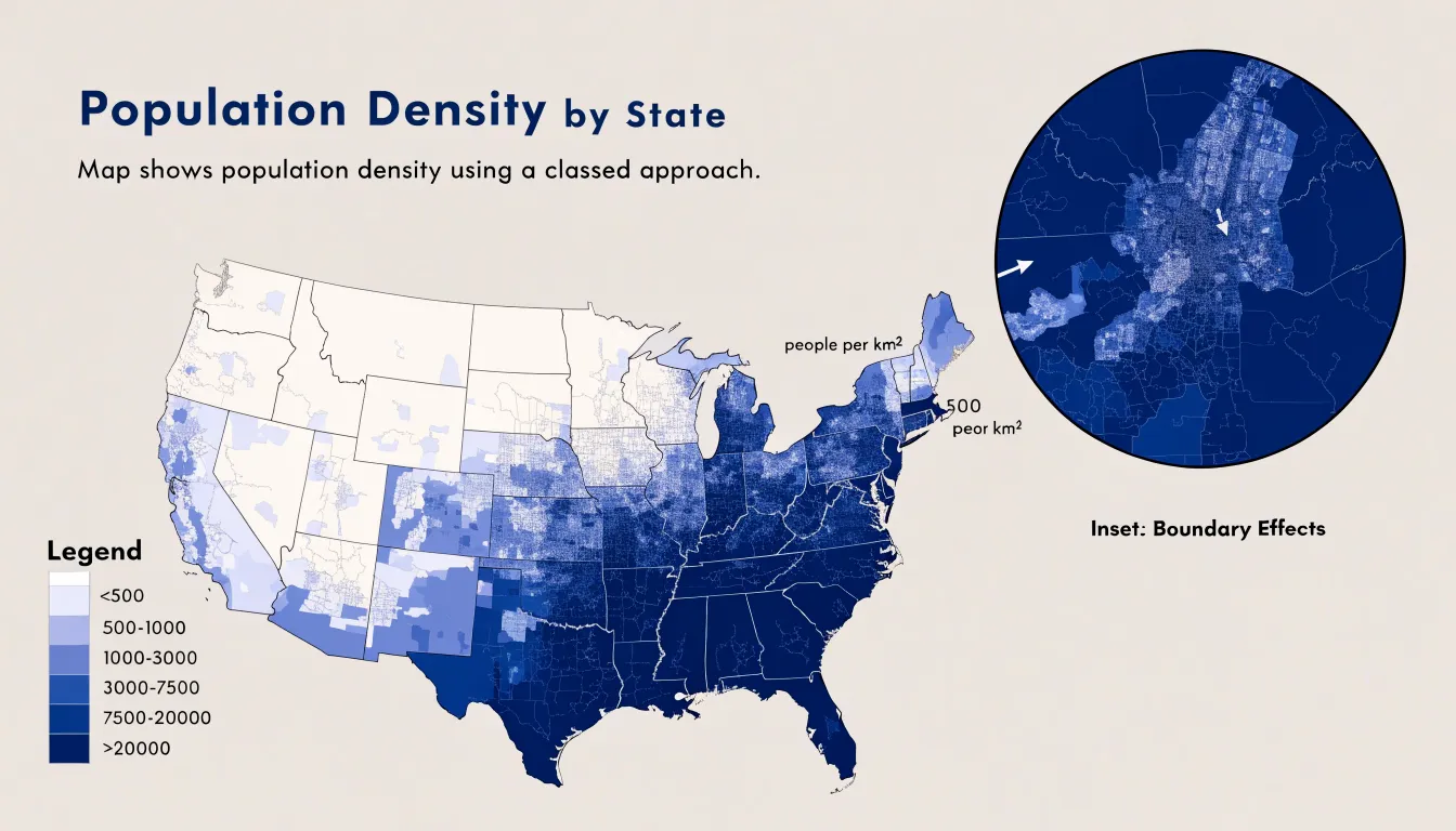
Accuracy in a choropleth map depends on sound choices about data classification and boundary definition. Analysts typically group density values into classes, such as equal intervals, quantiles, or natural breaks, and the chosen method shapes which regions stand out. Natural breaks tend to emphasize genuine gaps between dense and sparse zones, while quantiles spread colors more evenly across the map. Boundary selection matters just as much: large administrative units can average together a bustling city center and its empty hinterland, masking internal variation. Using smaller units, such as districts or census blocks, produces a finer picture of where density actually concentrates.
Color selection also influences interpretation. Sequential palettes that move from pale to saturated hues communicate ordered magnitude clearly, and they remain legible for readers with color vision deficiencies when contrast is carefully managed. A legend showing the numeric ranges behind each shade keeps the map honest and comparable across regions.
Well-constructed choropleth maps reveal familiar patterns: dense cores around major urban centers, gradual thinning toward suburbs, and broad light-toned expanses across rural territory. Planners, demographers, and general audiences can use these maps to spot underserved areas, anticipate infrastructure demand, or simply understand the human geography of a region at a glance.
Line Graphs
Line graphs serve as a natural fit for demographic metrics that unfold continuously across time, particularly birth and death rates measured over multiple decades. When a demographic indicator is plotted as a line moving from left to right along a chronological axis, readers can follow the trajectory of fertility and mortality as a single connected narrative rather than a series of disconnected annual figures. This continuity makes it easier to perceive the direction and pace of change: a gently declining line signals a gradual reduction in fertility, while a steep downward slope draws attention to an accelerated drop that may correspond with economic shifts, policy interventions, or changing social norms around family size.
The same principle applies to mortality. A sharp upward spike in a death-rate line stands out immediately against the surrounding baseline, flagging events such as epidemics, famine, conflict, or health-system crises. Because the line preserves the surrounding years as context, viewers can compare the height and duration of a spike against normal variation and judge how quickly mortality returned to prior levels. Multiple lines can be placed on a single chart to compare birth and death trends side by side, showing the widening or narrowing gap between them and revealing the demographic transition as it unfolds.
Effective line graphs for this purpose depend on a consistent time interval along the horizontal axis, clearly labeled units for the vertical axis, and a limited number of lines so that each trend remains legible. Annotations marking notable historical events help connect the shapes of the curves to their likely causes, turning a simple plotted line into an explanatory tool for understanding long-run population dynamics.
Grouped Column Charts
A grouped column chart is well suited to comparing employment status across regions because it places discrete labor categories side by side within each geographical jurisdiction. In practice, each region receives its own cluster of columns, and within that cluster a separate column represents a labor category such as employed full-time, employed part-time, unemployed, or outside the labor force. This arrangement lets readers move between two levels of analysis at once. Scanning horizontally across the chart, a reader can track how a single employment category performs from one region to the next. Scanning within a single cluster, the reader can see the internal composition of the workforce in that area. Both readings happen without switching charts, which keeps the comparison immediate and intuitive.
The side-by-side structure makes disparities visible at a glance. If one region shows a noticeably taller unemployed column relative to its neighbors, or a shorter full-time employment column, that gap stands out as a visual signal worth investigating. Analysts can use these signals to frame questions about local labor markets, industrial composition, or policy differences. Consistent color coding across clusters reinforces the comparison, so the same category reads the same way in every region.
Design details matter for clarity. Keep categories in a consistent order within each cluster, give columns a shared baseline, and label axes clearly so that regional names and labor categories are unambiguous. When many regions or categories are involved, consider splitting the chart into panels or highlighting a focal region. Handled with care, the grouped column chart turns a complex matrix of regions and employment statuses into a readable visual summary that supports evidence-based discussion of economic disparity.
Scatter Plots
Scatter plots place individual demographic records as points along two continuous axes, and this makes them a natural fit for exploring the relationship between educational attainment and income. Each point in the plot can represent a single person or a small group, with one axis carrying a measure such as years of schooling, highest credential earned, or average education level, and the other axis carrying a corresponding income figure like annual wage, hourly earnings, or household income. With the raw observations laid out in this way, readers can see the full shape of the data rather than a single summary number. The pattern that emerges often shows a general upward drift, where higher levels of education correspond to higher wages, and the scatter of points around that drift conveys how much variation exists among people at the same education level.
Scatter plots also let analysts examine the strength and form of a statistical relationship. A tight clustering of points along an upward path suggests a strong association, while a wide cloud of points suggests that education explains only part of the variation in pay. The plot can reveal whether the relationship looks linear or curved, whether it flattens at higher credential levels, and whether particular combinations produce unusual outcomes. Demographic attributes can be encoded through point color or shape, allowing comparisons between groups such as regions, age bands, or gender categories within the same frame. Showing individual observations supports transparency, since outliers and clusters remain visible and can be investigated directly.
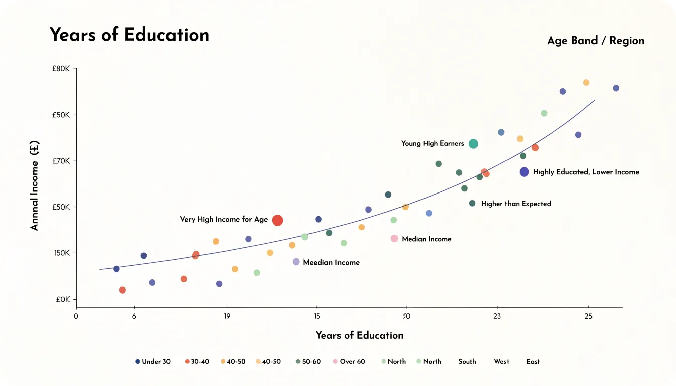
The approach works best when data points are plotted at a meaningful unit of analysis and axis scales are labeled clearly. With education on one axis and income on the other, a scatter plot turns a broad question about the value of schooling into a visual pattern that readers can interpret at a glance.
Dot Density Maps
Dot density maps translate demographic data into individual marks placed across a geographic space, with each dot representing a set number of residents from a particular racial or ethnic group. Within a local census tract, these dots are distributed across residential areas, streets, and blocks, giving viewers a fine-grained picture of how different populations share or occupy space at the neighborhood level. A tract that appears uniformly mixed in a choropleth map can reveal striking internal structure once rendered as dots, with clusters of one group concentrated on certain blocks and other groups dominating adjacent streets. This granularity makes dot density maps especially useful for examining integration patterns, since they show whether groups live in close proximity or remain separated by invisible boundaries within the same tract.
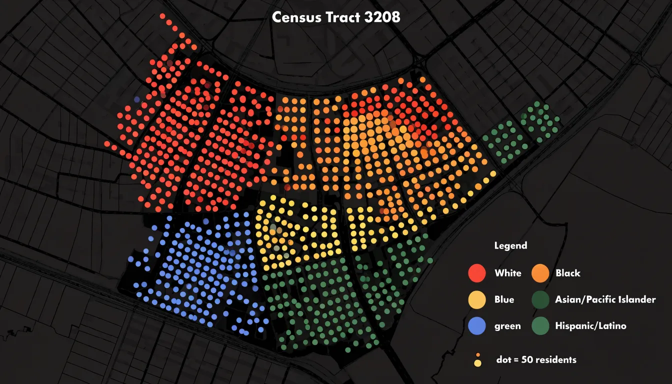
Designers control dot size, placement, and randomization to balance visual clarity with accuracy. Because census data is typically aggregated to blocks or block groups, the placement of dots within those units involves a degree of spatial approximation, and the chosen dot value determines how dense or sparse the final pattern appears. Overplotting becomes a concern in densely populated areas, where dots may merge into solid masses; adjusting dot size and using subtle transparency helps preserve readability. Color choices matter as well, since overlapping or adjacent dots from different groups need to remain distinguishable at small scales.
These maps work best when paired with clear legends explaining dot values and when applied to areas with sufficient population density to produce meaningful patterns. In practice, they give planners, researchers, and general audiences an intuitive sense of neighborhood diversity that aggregate statistics alone cannot convey, making visible the local texture of demographic mixing across the urban landscape.
Treemaps
Treemaps offer a distinctive way to present education levels through organized blocks, using nested rectangular spaces that visually encode both hierarchy and magnitude. Each rectangle represents a category of educational attainment, and the area of the rectangle corresponds directly to that category’s share of the total population. The largest blocks immediately draw the eye to the most common attainment levels, while smaller rectangles reveal the less frequent categories that might otherwise be lost in a conventional table. This proportional sizing makes it easy to compare how populations distribute across categories such as primary education, secondary education, vocational training, and tertiary degrees without requiring readers to perform mental arithmetic.
The nested structure of a treemap adds another layer of interpretive value. Subcategories can be nested within broader groupings, so that, for example, different levels of higher education sit inside a single tertiary block. This arrangement mirrors the hierarchical nature of education systems themselves, where certificates, diplomas, and degrees build upon one another. Viewers can scan the overall composition at a glance and then drill into the finer subdivisions that explain it. Color can reinforce these groupings, distinguishing one attainment band from another while keeping the overall layout compact and readable.
Treemaps work particularly well when demographic data must fit into a limited space, such as a dashboard or a printed report. They handle many categories gracefully and maintain consistent proportions across different population sizes, which supports comparisons between regions or cohorts. The block-based layout also lends itself to labeling, with larger rectangles carrying full text and smaller ones using abbreviations or legends. The result is a chart that turns abstract education statistics into a structured, visually organized map of the population.
Bubble Charts
A bubble chart extends the familiar scatter plot by introducing a third visual dimension through the size of each plotted marker. In demographic work, this makes it possible to place two core measures on the horizontal and vertical axes while reserving area for a variable that describes the scale of each group. A common application compares life expectancy against median income, with each point representing a country, region, or community. Position on the chart reveals the relationship between longevity and economic resources, while the diameter of the bubble communicates total group population size. Readers can immediately see whether large populations cluster in particular performance zones, such as high-income and high-longevity areas, or whether they are scattered across the chart.
Scaling bubbles accurately requires care. Area should be proportional to the underlying value rather than the radius, because human perception judges the size of a circle by its surface. When the population range is very wide, a linear scale may produce tiny bubbles alongside enormous ones. A square-root transformation of the radius often keeps the chart readable while preserving honest relative comparisons. A short legend showing reference circles, for instance populations of one million, ten million, and one hundred million, gives viewers a calibration point for interpreting the markers.
Colour and labels can add a further layer without overwhelming the display. Grouping bubbles by continent or income tier helps reveal patterns within the overall cloud of points, and annotating a handful of notable cases draws attention to outliers or exemplars. Overlapping bubbles present the main practical challenge, particularly where many small groups sit close together. Transparent fills, careful ordering of markers, and interactive tooltips in digital versions can mitigate this issue. The result is a compact visual summary that links three demographic measures in a single view.
Sankey Diagrams
Sankey diagrams offer a distinctive way to map population movements by representing each region as a node and each migration pathway as a flowing band whose width corresponds to the volume of people moving along it. When applied to demographic data, this visual format turns abstract relocation statistics into a readable picture of where people come from and where they go. A node on the left might represent a country of origin, while nodes on the right represent destination countries, and the connecting flows thicken or thin according to the number of migrants traveling that route. Readers can trace a single stream from a rural province to a coastal metropolis, or follow an international corridor linking one nation to another, and immediately grasp the relative scale of each movement.
For domestic relocation patterns, Sankey diagrams excel at showing the interplay between internal regions. A country experiencing urbanization can display streams from rural districts flowing into major cities, with the band widths revealing which source areas contribute most heavily to in-migration. Simultaneously, smaller counter-flows can be rendered alongside the dominant currents, capturing the return migration or suburban spillover that often accompanies large-scale internal shifts. This side-by-side presentation helps analysts identify net gainers and net losers among regions without resorting to dense tables.
International migration benefits from the same clarity. A diagram can set multiple origin countries against multiple destination countries, allowing viewers to compare corridors such as labor migration routes, refugee pathways, or family reunification flows. Because Sankey layouts preserve the total volume passing through each node, they also reveal intermediate hubs and transit countries that might otherwise go unnoticed in a simple bilateral comparison. The result is a compact visual summary that communicates both the direction and the magnitude of human movement, making complex relocation dynamics accessible to policymakers, researchers, and general audiences alike.
Violin Plots
Violin plots offer a rich way to examine income spread and variance across demographic groups by combining the summary structure of a box plot with a kernel density estimate on each side of the central axis. The resulting shape shows where values cluster and how far they stretch, so a reader can see the full distribution of income within each subgroup at a glance. The width of the violin at any given income level reflects how many observations sit near that value, while the symmetry around the centerline gives a mirrored density profile that is easy to compare across categories.
This combination is especially useful for revealing multimodal distributions. A group whose incomes cluster around two distinct ranges, such as entry-level wages and senior salaries, produces a violin with two bulges rather than a single smooth swell. A traditional box plot would flatten that structure into a median and a few quartiles, hiding the second peak entirely. The kernel density estimate preserves those separate concentrations and makes them visible, which helps analysts spot subpopulations that a summary statistic would obscure.
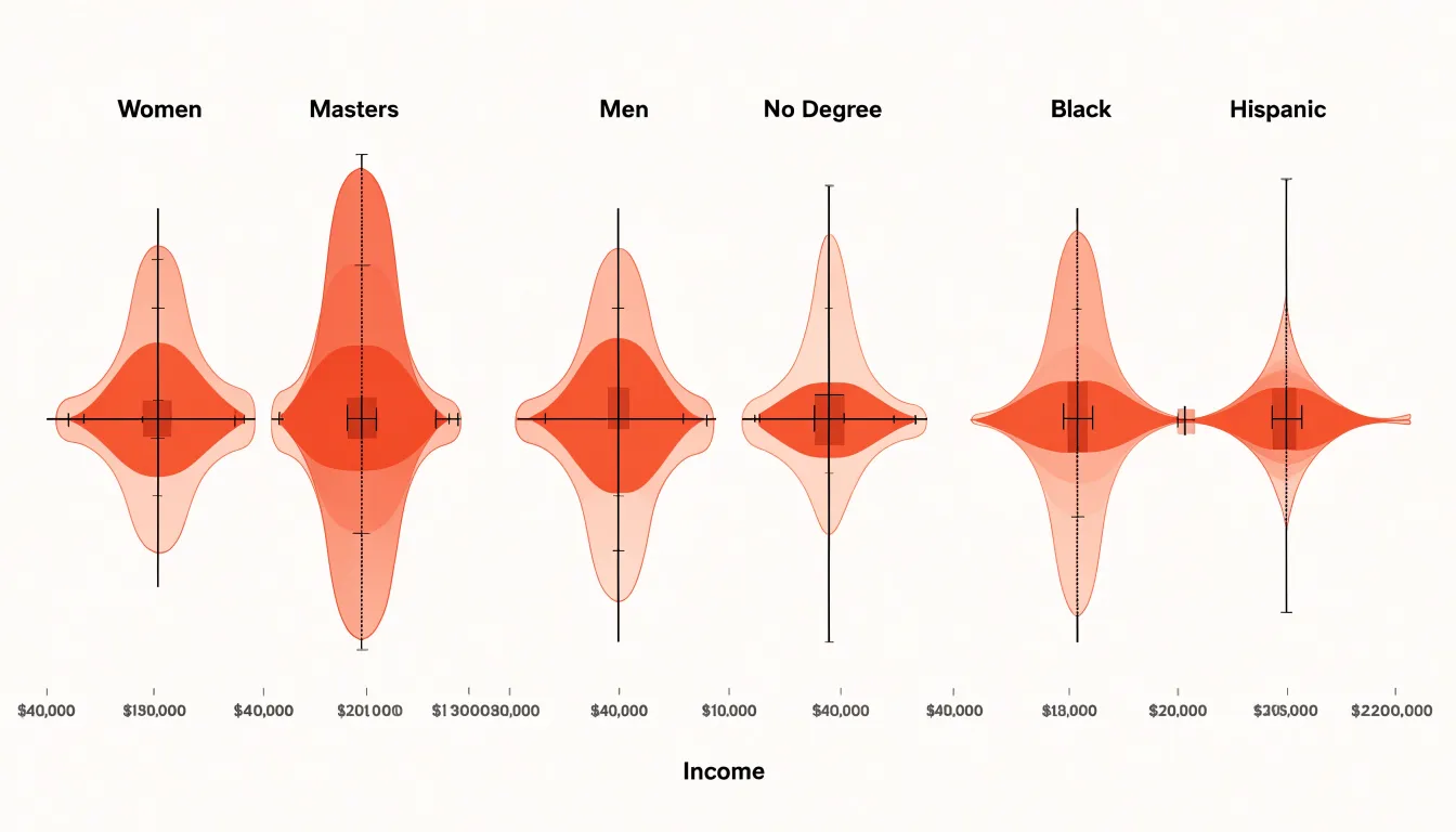
Violin plots also communicate income inequality within and between groups. A long, narrow tail toward high incomes signals a small number of very large earners pulling the distribution upward. A wide, short violin indicates incomes packed tightly around a central value. By placing violins for several demographic subsets side by side, viewers can compare medians, interquartile ranges, and tail behavior in a single view, seeing which groups have greater internal dispersion and which are more homogeneous. The mirrored density also makes skewness apparent, since an asymmetric violin shows incomes piling toward one end of the scale. Used carefully with clear labeling and consistent scaling, violin plots give demographic analysts a compact visual summary that captures spread, shape, and the presence of multiple income clusters across groups.
Waffle Charts
A waffle chart uses a 10x10 grid of one hundred small squares to display a simple proportion. Each square stands for one percent of a total population, so a group making up 30 percent of a population fills thirty squares in a contrasting color while the remaining seventy stay in a neutral shade. This arrangement turns an abstract percentage into a counted quantity that a reader can verify at a glance by tallying squares. For demographic communication aimed at broad audiences, this quality matters, because many readers process a concrete count of visible marks more readily than a decimal figure or an unfamiliar ratio.
The format suits simple proportional metrics particularly well. When a report needs to show what share of a population belongs to a single category, such as the percentage of residents born outside the country or the proportion of households with children, a waffle chart presents that figure as the dominant visual element. The ten-by-ten structure provides a natural reference frame, since most viewers already associate the full grid with the whole, and partial grids with parts of it. Small multiples extend this logic: placing several waffle charts side by side allows comparisons across regions or years while each individual graphic remains easy to read.
Waffle charts also work well in settings where the audience is diverse in background and data literacy. The grid avoids the interpretive demands of pie slices, whose angles are hard to compare, and the abstraction of bar lengths, which can obscure the underlying population. A colored square corresponds directly to a person or household in the aggregate, giving the chart a pictographic quality that supports intuitive reading. Simple rounding keeps the display honest, and filling squares in a consistent order from the top left supports quick scanning. For communicating one or two headline percentages to a general readership, the waffle chart delivers clarity with minimal explanation.
Dashboard Design Principles
Effective demographic dashboards balance information density with clarity, ensuring users can explore patterns without feeling overwhelmed. A well-structured layout typically follows a hierarchy: place the most critical demographic indicators, such as population pyramids or age-sex distributions, in prominent positions like the top-left or center, where they draw immediate attention. Secondary charts, like regional comparisons or trend lines, should occupy supporting areas, grouped logically by theme or geography. Use a grid system to align charts and maintain consistent spacing, which reduces visual clutter and guides the eye naturally from one element to the next. Interactive elements—filters, tooltips, and cross-highlighting—should be intuitive; for instance, clicking a segment in a pie chart could filter other charts to show only that subgroup, enabling seamless drill-down without requiring users to learn complex controls.
Color consistency is equally vital. Assign a fixed color palette to demographic categories (e.g., blue for males, orange for females) and apply it uniformly across all charts. This consistency leverages preattentive processing, allowing users to quickly associate colors with groups and compare across visuals. Avoid using too many hues; limit the palette to 5–7 distinct colors and use saturation or lightness variations for subcategories. Ensure sufficient contrast for readability and consider colorblind-friendly schemes. Consistency also extends to legends and labels—place them in standard locations and use identical terminology throughout.
Preventing cognitive overload requires thoughtful restraint. Limit the number of charts on a single screen to 5–7, and avoid overcrowding with unnecessary decorations. Use progressive disclosure: start with high-level summaries and allow users to reveal details on demand. For example, a map might show overall population density, with hover interactions revealing age breakdowns. Simplify chart types—prefer bar charts for comparisons and line charts for trends—and avoid 3D effects or excessive gridlines. Provide clear titles and brief annotations to guide interpretation. Finally, test the dashboard with representative users to identify confusion points and refine the layout iteratively. By adhering to these principles, demographic dashboards become powerful tools for insight discovery rather than sources of frustration.
Frequently Asked Questions
What does a population pyramid show?
A population pyramid is a dual-axis bar chart with males on one side and females on the other, where each horizontal bar represents an age cohort. Its shape shows population structure, such as a broad base indicating a youth bulge or a narrow base with wider middle or upper bars signaling an aging population.
How do I make a stacked bar chart easier to read?
Order segments consistently across every bar, keep the largest or most conceptually central group at the base, and use the same color for a group everywhere it appears. If there are too many segments, merge small categories into an aggregated remainder or show a limited set of key groups and note the consolidation in a caption.
Why does data classification matter in a choropleth map?
Analysts group density values into classes such as equal intervals, quantiles, or natural breaks, and the chosen method shapes which regions stand out. Natural breaks tend to emphasize genuine gaps between dense and sparse zones, while quantiles spread colors more evenly across the map.
When should I use a line graph for demographic data?
Line graphs fit demographic metrics that unfold continuously across time, particularly birth and death rates measured over multiple decades. They let readers follow the trajectory of fertility and mortality and compare trends when multiple lines are placed on one chart.
What is a grouped column chart good for?
A grouped column chart is well suited to comparing employment status across regions because it places discrete labor categories side by side within each region’s cluster. Readers can scan across regions for one category or within a cluster to see the internal workforce composition.
How do dot density maps show neighborhood diversity?
Dot density maps place individual marks across a geographic space, with each dot representing a set number of residents from a particular racial or ethnic group. Within a census tract, these dots are distributed across residential areas, streets, and blocks, revealing fine-grained clustering and integration patterns that a choropleth may not show.
Tony Astor
Tony writes about data visualization and the tools people use to build charts and dashboards. More about Data Illustrator