Best Charts for Climate and Weather Data
 By Tony Astor ·
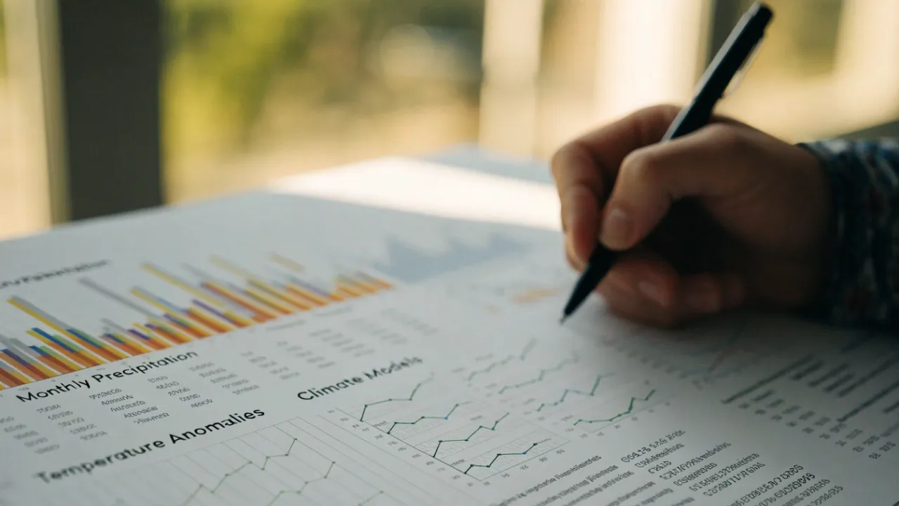
Best Charts for Climate and Weather Data
The best charts for climate and weather data include temperature trend lines for long-term warming, precipitation bar graphs for seasonal rainfall, heatmap matrices for spotting anomalies, wind rose diagrams for directional wind patterns, sea level rise area charts, streamgraphs for air quality, scatter plots for humidity, isohyetal contour maps for rainfall distribution, box plots for seasonal temperature ranges, bubble maps for carbon emissions, dual axis climographs, hurricane track maps, and interactive dashboards.
Table of Contents
- Temperature Trend Lines
- Precipitation Bar Graphs
- Heatmap Matrices
- Wind Rose Diagrams
- Sea Level Rise Area Charts
- Streamgraphs for Air Quality
- Scatter Plots for Humidity
- Isohyetal Contour Maps
- Box Plots for Seasonal Temps
- Bubble Maps for Carbon Output
- Dual Axis Combination Charts
- Hurricane Track Line Maps
- Interactive Climate Dashboards
Temperature Trend Lines
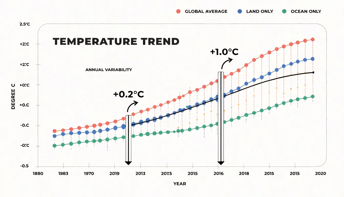
Temperature trend lines serve as a powerful way to visualize how global temperatures have shifted over decades, making them essential for anyone working with climate and weather data. Simple multi-line graphs can display several temperature series side by side, such as global averages, land-only readings, and ocean-only measurements, letting readers compare how each has evolved across the same time span. When these lines are plotted over long horizons, the upward drift becomes immediately visible, even though individual years fluctuate up and down. Adding a moving-average line on top of the raw annual values smooths out short-term noise from events like El Niño or volcanic eruptions, revealing the underlying direction of change. This combination of raw data and smoothed trend gives viewers both detail and clarity. Surface warming anomalies are especially well suited to this format, since plotting deviations from a baseline period rather than absolute temperatures makes shifts easier to spot and compare across regions. Multi-decade climate shifts, such as the acceleration of warming in recent decades, stand out clearly when trend lines are extended across the full historical record. Designers can strengthen these charts by annotating key milestones, using consistent color palettes for each series, and labeling axes with clear units. A well-built trend line chart communicates the story of a warming planet at a glance, turning thousands of data points into a single, readable narrative that supports both scientific communication and public understanding.
Precipitation Bar Graphs
Precipitation bar graphs organize rainfall totals into discrete columns, and when those columns are grouped by month, they become a compact visual record of how wet and dry periods alternate through the calendar year. A grouped bar chart typically places months along the horizontal axis and rainfall depth along the vertical axis, with separate bars for each location or year drawn side by side within every month. This arrangement makes seasonal rhythm immediately legible: a reader can see the columns rise through spring, peak in midsummer, and fall away in autumn without needing to consult a table. Stacked bars work on the same framework, dividing each monthly column into segments that represent individual storm events, rainfall intensity bands, or contributions from different monitoring stations, so the total height still communicates the monthly aggregate while the internal structure reveals how that total accumulated. These charts handle drought spells particularly well, since a run of unusually short columns stands out against the surrounding seasonal context and signals a sustained rainfall deficit rather than a single dry week. Extreme monsoon events appear as dramatic spikes, and the grouping makes it possible to compare the magnitude of a deluge in one region against the same month in another, exposing how monsoon onset and intensity shift with latitude, elevation, or proximity to coastlines. Placing several geographic regions in one grouped chart supports direct comparison across shared months, which helps analysts identify which areas face synchronized wet seasons and which experience offset rainfall calendars. The categorical month axis also accommodates annotations for thresholds such as flood-stage rainfall or agricultural water requirements, turning the bar graph into a decision-support tool for water managers, farmers, and emergency planners who need to spot recurring risk windows at a glance.
Heatmap Matrices
Heatmap matrices transform dense climate data into an immediate visual language where color intensity reveals patterns that tables of numbers would obscure. By mapping temperature values to a color gradient across a grid of geographic coordinates and time periods, these matrices allow analysts to scan for anomalies at a glance. For instance, a global temperature dataset spanning decades can be rendered as a matrix with latitude and longitude on one axis and months or years on the other. The result is a vivid tapestry where warm hues cluster in specific regions, instantly highlighting areas experiencing sustained heatwaves or anomalous warming trends.
This approach is particularly effective for identifying urban heat islands. When high-resolution data is plotted in a matrix, cities emerge as distinct hot spots against cooler surrounding rural areas, even when the overall regional temperature is moderate. Planners can use such visualizations to target mitigation strategies, such as increasing green spaces or reflective surfaces, in the most affected neighborhoods. Similarly, heatmap matrices excel at revealing abnormal weather anomalies, such as sudden spikes in temperature or precipitation, by contrasting them against the expected baseline color. A deviation in the matrix stands out as a stark color shift, prompting further investigation.
The strength of heatmap matrices lies in their ability to handle high-density datasets without clutter. Each cell represents a specific combination of location and time, and the color encodes the value, enabling the simultaneous comparison of thousands of data points. This makes them invaluable for climate monitoring, where spotting a localized surge quickly can inform early warnings or resource allocation. By leveraging the human visual system’s sensitivity to color differences, heatmap matrices convert complex climate data into actionable insights, empowering researchers and decision-makers to respond swiftly to emerging hotspots and anomalies.
Wind Rose Diagrams
Wind rose diagrams use a polar coordinate layout to show how often the wind blows from each direction at a monitoring station and how fast those winds typically move. The compass directions around the circle serve as the categorical axis, with north at the top and the remaining directions spaced evenly around the perimeter. Each direction sector contains a stacked set of colored bands, and each band represents a range of wind speeds. The length of a sector reveals how frequently the wind arrived from that direction during the chosen timeframe, while the order of the colored bands shows velocity, with calm or light winds near the center and stronger winds extending toward the outer edge. A station where long sectors cluster to the southwest will read at a glance as a place dominated by southwesterly airflow, while a circular, evenly spread pattern signals varied conditions with no strong prevailing direction.
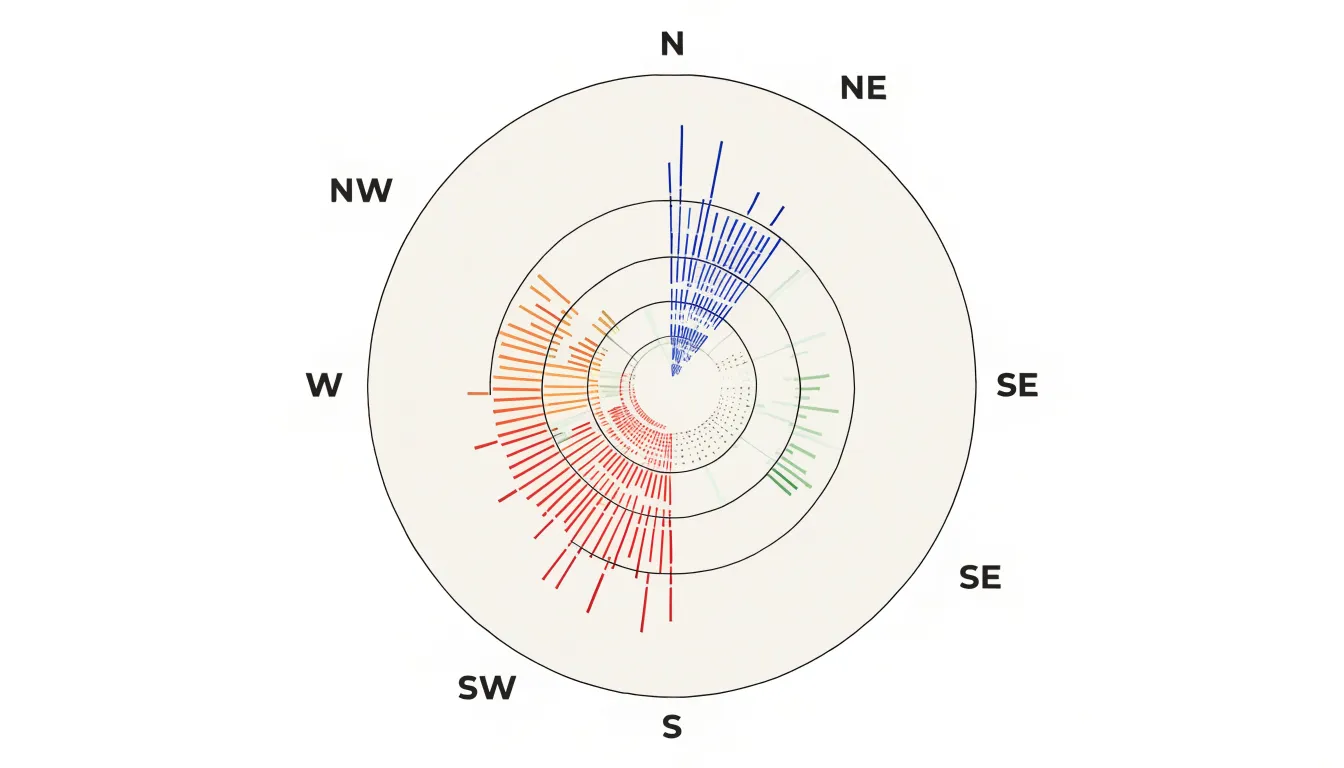
For climate and weather work, the chosen timeframe matters a great deal. Analysts can build a wind rose from a single season, a year, or a multi-decade record to see how local breezes shift over time. Coastal stations show the influence of sea and land breezes, mountain sites reveal valley drainage flows, and urban stations expose channeling between buildings. The proportional radius of each speed band also makes it easy to compare the frequency of gale-force winds against gentler daily movement. Placing several wind roses side by side lets readers compare neighboring stations or contrast one period against another and spot changes in prevailing direction or storminess. Because the visual language is compact and instantly legible, wind roses serve well as summary graphics within larger climate reports and dashboards.
Sea Level Rise Area Charts
Sea level rise area charts use filled area graphs to trace how coastal baseline water levels have shifted across decades of measurement, and they belong to the family of cumulative time-series visuals that make long-term change legible at a glance. In these charts, the vertical axis represents measured water height or cumulative oceanic volume, while the horizontal axis carries the timeline of observations, often stretching back to the late nineteenth century when reliable tide gauge records began. The filled space beneath the line draws the eye to the total accumulation rather than to isolated datapoints, so a reader can see how each decade builds on the last.
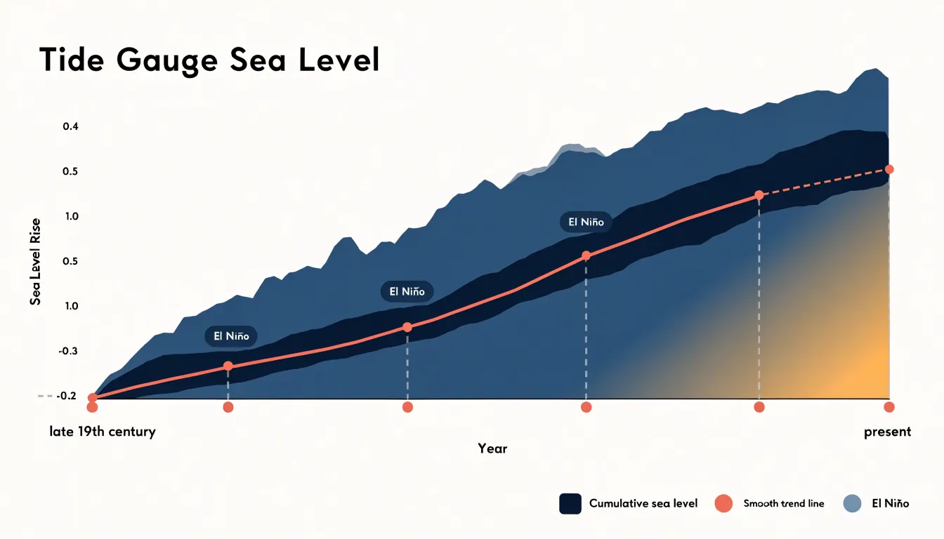
Tide gauge metrics are the raw material for most of these visualizations. Coastal stations around the world record the mean high water mark, and area charts aggregate those readings into a single sweeping band that rises steadily from left to right. Where satellite altimetry data overlaps with gauge records, the fill can be layered to show agreement between the two measurement systems and to extend the curve into the present day. Because the area beneath the curve is shaded, the chart communicates volume as well as height, giving viewers an intuitive sense of how much water has accumulated over the recorded period.
The dramatic character of the rise emerges through the shape of the curve itself. A baseline that appears nearly flat across the early twentieth century begins to steepen noticeably in the latter half of the century, and the filled band thickens rapidly toward the right edge of the chart. Annotations for major flooding events or for years with strong El Nino influence can be overlaid to explain short-term spikes without obscuring the long-term trend. Smoothed trend lines drawn across the fill help separate the underlying signal from year-to-year noise.
For coastal planners, these charts translate abstract measurements into a tangible picture of creeping shorelines. A filled area graph showing a meter of rise over a century reads as a visible inundation of the space beneath the line, which makes the stakes of adaptation planning concrete for audiences who might otherwise struggle to interpret raw tide gauge tables.
Streamgraphs for Air Quality
Streamgraphs offer a distinctive way to follow air quality through the calendar year, especially when several pollutants need to be watched at once. Their flowing, stacked bands show the volume of each component while also revealing how the overall mix shifts month by month. When plotting PM2.5, ozone, and nitrogen dioxide together, the graph creates a continuous ribbon of information where the relative thickness of each layer tells the story of which pollutant dominates at any given time.
The appeal of this chart type lies in its emphasis on movement. Pollution does not sit still; it rises and falls with the seasons, driven by heating patterns, weather systems, and changes in traffic or industrial activity. A streamgraph captures that rhythm. Winter months often show PM2.5 thickening as domestic heating and stagnant air trap particulates near the ground. Spring and summer can bring ozone to the foreground, with its bands widening during sunny, high-temperature periods when photochemical reactions accelerate. Nitrogen dioxide tends to track traffic and combustion sources, and its band may swell during rush-hour-heavy months or shrink during holiday lulls.
Because the bands are centered on a flowing axis, streamgraphs make it easy to spot the moments when one pollutant surges relative to the others. A sudden bulge in the PM2.5 layer during a wildfire season or a winter inversion becomes immediately visible against the surrounding flow. These visual spikes draw attention to the periods when air quality poses the greatest health risk and invite closer investigation of the conditions behind them.
The fluid design suits the cyclical nature of atmospheric data. Rather than presenting a rigid grid or a cluster of separate lines, the streamgraph shows the year as a continuous, changing landscape of pollutants. For readers trying to understand seasonal air quality patterns, this makes the chart both informative and engaging.
Scatter Plots for Humidity
Scatter plots provide a direct way to examine how moisture variables move in relation to temperature. By placing ambient temperature on one axis and a humidity measure such as dew point or relative humidity on the other, each observation becomes a single point in a two-dimensional field. The resulting cloud of points reveals patterns that summary statistics alone can obscure, including the direction, strength, and shape of the relationship between heat and moisture.
Dew point is especially well suited to this treatment because it tracks the absolute amount of water vapor in the air and stays relatively stable through the daily temperature cycle. Plotting dew point against temperature often produces a clustering pattern: most observations fall within a characteristic band, while a smaller number of points sit above or below it. Those outliers flag air masses with unusually high or low moisture content, which forecasters can follow as they track changes in the coming hours.
Relative humidity behaves differently in a scatter plot. Because it depends on temperature, the two variables typically trace a curved, inverse relationship, with high relative humidity concentrated at cooler temperatures and lower values spreading out as heat builds. The curvature itself is informative, since it shows where small temperature changes translate into large shifts in saturation deficit.
The practical value lies in heat index forecasting. Heat index combines temperature and humidity into a single measure of apparent temperature, and the severity of that combined effect depends on where an observation falls within the scatter pattern. Points in the upper-right region of a dew point versus temperature plot signal hot, muggy conditions capable of pushing heat index values into dangerous territory, while points along the lower edge suggest drier heat with a milder apparent temperature. Reading these positions across successive observations helps forecasters anticipate when oppressive conditions will intensify and communicate risk more precisely to the public.
Isohyetal Contour Maps
Isohyetal contour maps use continuous lines to connect points of equal rainfall, transforming scattered gauge readings into a coherent picture of how precipitation is distributed across a region. Each contour, or isohyet, traces a boundary where the same rainfall total was recorded, and the spacing between successive lines reveals the steepness of the precipitation gradient. Where isohyets crowd closely together, rainfall changes rapidly over short distances; where they spread apart, totals shift gradually across the landscape. This visual grammar lets readers trace storm rainfall across geography at a glance, following bands of heavy precipitation as they extend over valleys, ridges, and coastal plains.
The technique draws on the same cartographic logic as topographic maps, and its power lies in how it reconciles point measurements with continuous terrain. Rain gauges and radar estimates provide values at discrete locations, and the contouring process interpolates between them to suggest how much rain likely fell in the unmeasured spaces between. By overlaying these contours on elevation models, analysts can show how topography shapes precipitation: mountain ranges wring moisture from passing systems, creating tight clusters of high-value isohyets on windward slopes, while rain shadows appear as wider spacing and lower totals on the leeward side. Storm tracks emerge as elongated patterns of nested contours, with a core of maximum rainfall surrounded by concentric rings of decreasing totals.
Isohyetal maps serve forecasters, hydrologists, and emergency planners who need to anticipate runoff, flooding, and water resource impacts. The contour lines convert raw precipitation volume into a readable gradient field, revealing where a storm delivered its heaviest load and how that load tapered off across the surrounding terrain.
Box Plots for Seasonal Temps
Box plots, also known as box-and-whisker diagrams, provide a concise statistical summary of temperature distributions for seasons or months, making them ideal for comparing variability and extremes across years or locations. Each box represents the interquartile range (IQR), from the 25th to the 75th percentile, capturing the middle 50% of daily temperatures. The horizontal line inside the box marks the median, while the whiskers extend to the lowest and highest values within 1.5 times the IQR. Any points beyond the whiskers are plotted individually as outliers, highlighting unusually hot or cold days that deviate from the typical range.
For climate analysis, this structure is particularly useful for tracking shifts in seasonal temperature baselines. By constructing side-by-side box plots for each year or decade, analysts can see whether the median temperature is rising, whether the IQR is widening or narrowing, and whether the frequency of outliers is increasing. A gradual upward shift in the median and a higher number of warm outliers, for example, indicate a warming trend. Similarly, a longer upper whisker in recent years suggests more frequent days with extreme heat.
Box plots also facilitate comparisons across multiple locations or seasons. Because they display key statistics without assuming a specific distribution, they are robust to non-normal data and outliers. This makes them well-suited for weather station records, which often contain anomalies. When used alongside time series or heatmaps, box plots add a layer of statistical depth, helping viewers quickly grasp how temperature extremes are changing and where the most significant shifts are occurring. Ultimately, they offer a compact yet powerful way to visualize the range and frequency of extreme temperatures, supporting informed decisions in climate adaptation and risk management.
Bubble Maps for Carbon Output
Bubble maps offer a way to place national greenhouse gas emissions directly onto the geography they originate from, using circles scaled by total emissions and positioned over each country’s territory or capital. The visual result lets readers see at a glance which regions carry the heaviest emissions burden while retaining the spatial context that a plain bar chart would strip away. Because the circle’s area encodes the emissions value, the size difference between a high-emitting nation and a low-emitting neighbor becomes immediately legible, even when the smaller country covers more land. Layering population density beneath the bubbles adds a second dimension: a large bubble over a densely populated area invites the reader to consider emissions per person, while a large bubble over a sparsely settled region points toward industrial or extractive activity as the driver. Land mass matters here as well, since a country with a vast territory may show moderate per-area density yet rank high in absolute emissions. Designers typically tune the scaling carefully so overlapping bubbles remain readable, sometimes allowing partial transparency or slight offset from the exact centroid. Color can encode a third variable, such as emissions per capita or growth trend, turning the map into a compact multi-variable display. The technique works best when the number of bubbles is manageable and the geographic base is not too crowded, and it rewards viewers who take a moment to compare circle areas rather than jumping to conclusions from color alone. Used thoughtfully, bubble maps connect the abstract numbers of national carbon accounts to the physical geography of the planet, making the distribution of emissions feel tangible and grounded in place.
Dual Axis Combination Charts
Dual axis combination charts pair two different chart types, most commonly bars and lines, on a shared horizontal axis while assigning each series its own vertical scale. In climate and weather analysis, this structure is the backbone of the classic climograph, where monthly rainfall appears as vertical bars and average temperature is traced as a continuous line across the same twelve-month timeline. The bar layer communicates volume and accumulation, showing how much precipitation falls in each period, while the line layer communicates trend and trajectory, revealing how temperature rises and falls through the seasons. Because rainfall is measured in millimeters and temperature in degrees Celsius, forcing both onto a single scale would flatten one series into near-invisibility or exaggerate the other beyond recognition. Separate vertical axes, clearly labeled and color-matched to their series, let each variable occupy its natural range so that patterns in both remain legible at a glance.
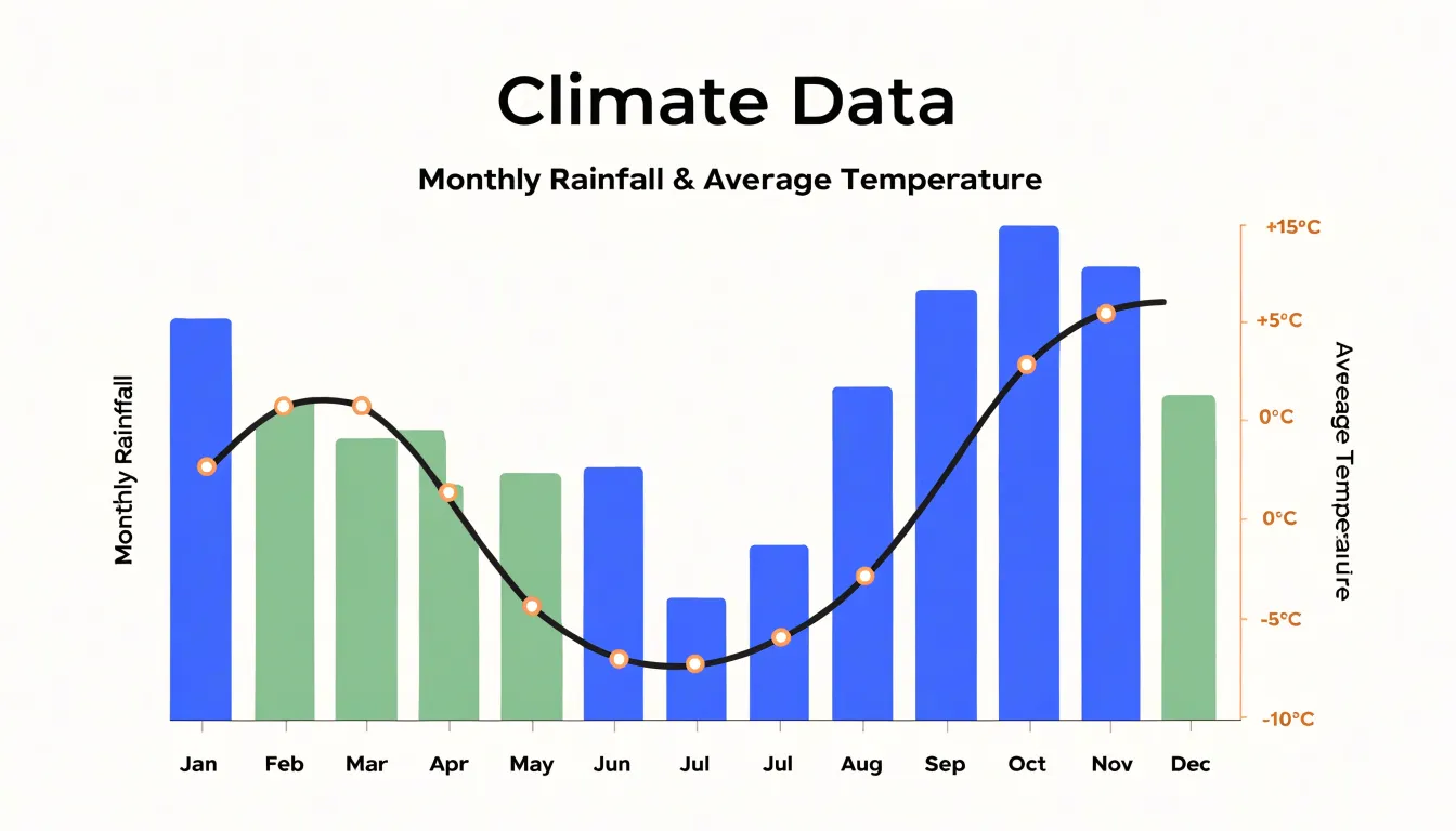
The analytical payoff comes from reading the two layers together. A viewer can spot the onset of a wet season against the backdrop of warming temperatures, identify dry spells that coincide with peak heat, and recognize the lag between maximum rainfall and maximum temperature that characterizes many tropical and monsoon climates. These co-dependent relationships matter for agriculture, water resource planning, and ecosystem monitoring, since the interaction between moisture and heat often determines outcomes more than either variable alone. Animated or interactive versions extend the technique further, allowing analysts to step through months or years and watch how the relationship between the bar and line layers evolves over time, making seasonal shifts and anomalous years immediately apparent.
Hurricane Track Line Maps
Hurricane track line maps give emergency planners a visual language for communicating where a tropical storm is heading and what it may do when it arrives. The backbone of these maps is the trajectory vector line, a continuous path that threads through forecast positions at set intervals. Each point along the line typically carries a timestamp, so a viewer can trace the storm’s projected movement hour by hour across the ocean basin. Vector lines often include an arrowhead or directional cue, making the forward motion of the system immediately legible even to audiences unfamiliar with meteorological conventions. Where the line crosses from open water toward a coastline, the map marks the anticipated landfall location, anchoring the abstract forecast to a specific stretch of shore.
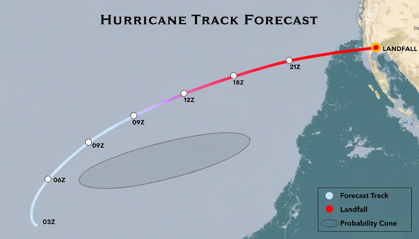
Intensity progression is layered onto the same graphic through color, size, or symbol changes along the track. A line that shifts from pale blue to deep red as it approaches land signals strengthening, while markers shaped like letters or spirals may designate tropical storm, hurricane, and major hurricane thresholds. These cues help planners anticipate surge heights, wind damage, and evacuation timing rather than treating the storm as a single undifferentiated threat.
Probability cones add a second dimension of information. The cone widens with forecast lead time, reflecting growing uncertainty in the storm’s future position. A narrow cone near the current location conveys high confidence, while a broad cone three or four days out shows that the landfall zone could span hundreds of miles. Emergency managers use this widening shape to decide when to issue watches, stage supplies, and prepare coastal communities across a range of possible outcomes. Combined with track lines and intensity markers, probability cones turn a hurricane forecast into an actionable planning instrument for coastal landfall risk.
Interactive Climate Dashboards
Interactive climate dashboards bring together temperature curves, precipitation bars, wind rose diagrams, and anomaly maps into a single, cohesive interface. Rather than reviewing these chart types in isolation, users can view them side by side or layered on top of one another, revealing relationships that would otherwise remain hidden. A researcher examining a drought period, for example, can simultaneously observe declining rainfall bars, rising temperature lines, and soil moisture heatmaps, building a richer picture of the conditions that produced the event. This unified presentation supports holistic environmental analysis because each chart type contributes a distinct perspective while the dashboard preserves the connections among them.
Real-time updates add substantial value to this approach. When dashboards pull live data from weather stations and satellite feeds, decision-makers work from current conditions rather than stale summaries. Emergency planners monitoring an approaching storm can watch wind speeds climb on a gauge chart while precipitation forecasts shift on a timeline, adjusting their response as the situation evolves. Agricultural managers use the same capability to time irrigation against real-time evapotranspiration readings and short-term rainfall projections.
Interactivity deepens the analytical experience further. Users can hover over data points to read exact values, filter by date range, zoom into regional detail, or toggle specific layers on and off. Comparative tasks become straightforward, such as placing this year’s temperature trajectory beside a historical baseline to assess deviation. Shared dashboards also improve communication across teams, since stakeholders with varying technical backgrounds can explore the same evidence through intuitive visual controls.
Combining multiple chart types within one responsive interface transforms scattered observations into an integrated decision-support tool, giving analysts, planners, and the public a practical way to interpret complex climate and weather information as it unfolds.
Frequently Asked Questions
What chart is best for showing long-term temperature trends?
Temperature trend lines are used to visualize how global temperatures have shifted over decades, especially when multiple series are plotted side by side. Adding a moving-average line can smooth short-term noise and reveal the underlying direction of change.
How do precipitation bar graphs show seasonal rainfall and drought?
Grouped precipitation bar graphs place months along the horizontal axis and rainfall depth along the vertical axis, making seasonal rhythm easy to see. A run of unusually short columns can signal a sustained rainfall deficit rather than a single dry week.
What are heatmap matrices used for in climate data?
Heatmap matrices map values such as temperature to a color gradient across a grid of geographic coordinates and time periods, allowing anomalies to be spotted at a glance. They are effective for identifying urban heat islands and abnormal weather anomalies while handling high-density datasets without clutter.
How do wind rose diagrams show wind direction and speed?
Wind rose diagrams use a polar layout with compass directions around the circle, and the length of each sector shows how frequently wind came from that direction. Colored bands within each sector represent ranges of wind speeds, with stronger winds extending toward the outer edge.
What chart can compare temperature and rainfall on the same timeline?
Dual axis combination charts pair two chart types, most commonly bars and lines, on a shared horizontal axis while giving each series its own vertical scale. In a climograph, monthly rainfall appears as vertical bars and average temperature is traced as a continuous line across the same timeline.
How are probability cones used in hurricane track maps?
Probability cones widen with forecast lead time to reflect growing uncertainty in a storm’s future position. Emergency managers use the widening shape to decide when to issue watches, stage supplies, and prepare coastal communities across a range of possible outcomes.
Tony Astor
Tony writes about data visualization and the tools people use to build charts and dashboards. More about Data Illustrator