Best Charts for A/B Test Results
 By Tony Astor ·

Best Charts for A/B Test Results
Bar charts are the best default for comparing A/B test conversion rates, since bar height maps directly to each variant’s rate and makes the gap versus control instantly readable. Use confidence interval plots to show how certain that result is, and add cumulative gain, significance, and sample size charts to judge stability and decide when to stop.
Table of Contents
Bar Charts
Bar charts offer one of the most direct ways to compare conversion rates between a baseline control group and one or more test variants. Each variant is represented by a bar whose height corresponds to its conversion rate, so the visual distance between bars translates immediately into the size of the performance gap. When the control bar sits beside the variant bar, readers can see at a glance whether the new version gained or lost ground and by roughly how much. This makes simple bar charts especially useful in reports where stakeholders need a fast, intuitive read of the headline result without working through tables of raw numbers.
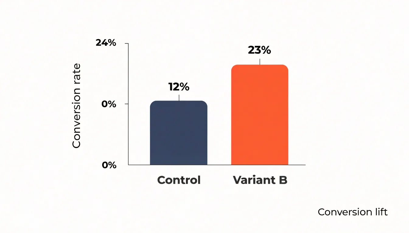
Grouped bar charts extend this approach to tests with more than two arms or with multiple segments. By placing bars side by side within each group, a grouped layout lets viewers compare several variants against the control while also comparing the same variant across different audiences, time periods, or devices. Color coding keeps the control consistent across groups, so the eye can track the baseline category from group to group and judge each variant against it in context. This structure works well when an experiment includes several challengers or when results are broken down by cohort.
Because bar height maps to a single percentage, these charts also make small differences visible in a way that summary sentences sometimes obscure. Adding data labels with the exact percentage on top of each bar pairs the quick visual impression with the precise figure, which supports both skimming and detailed review. Keeping the y-axis at a fixed scale across related charts preserves honest comparisons, and starting the axis at zero avoids exaggerating gaps between closely matched variants.
Confidence Interval Plots
A confidence interval plot takes the point estimate of your A/B test lift and surrounds it with a visual range that reflects how much that estimate could reasonably vary. In practice, this usually means drawing error bars around the observed difference between your control and variant groups, with the width of those bars determined by your chosen confidence level, typically 95 percent. The point in the middle represents the most likely value of the true effect, while the ends of the bars mark the boundaries of the range consistent with your data. This single visual immediately communicates something a bare percentage lift cannot: how certain the result really is.
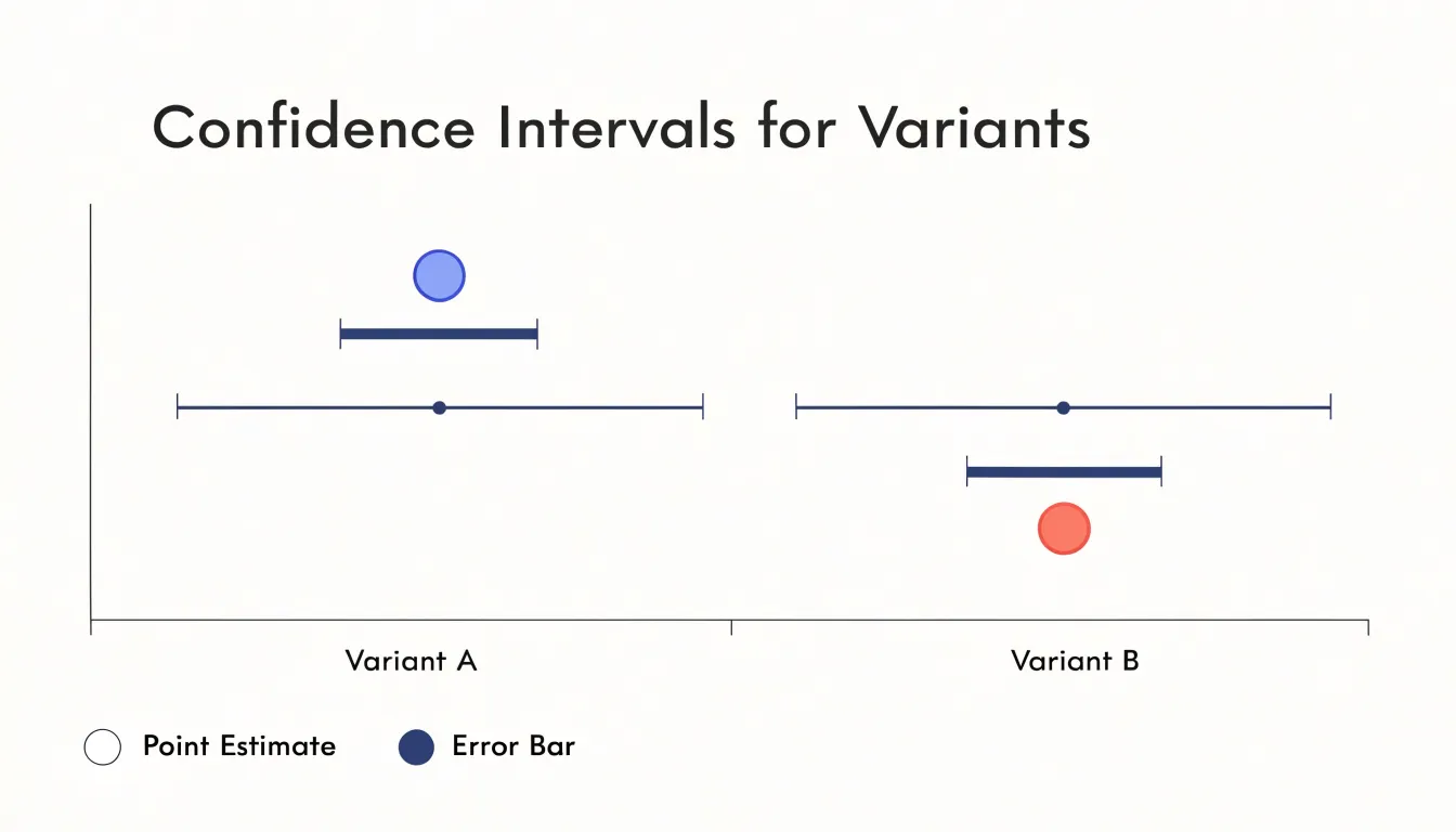
When readers see these bars, they can judge whether the observed winner is clearly separated from zero or whether the interval straddles it. A wide interval signals that the test simply did not collect enough data to pin down the effect, and any decision made on that estimate carries meaningful risk. A narrow interval suggests the estimate is stable and gives stakeholders confidence that the real-world lift will land close to what was measured. Plotting intervals for several metrics side by side makes these comparisons even more useful, since longer-running or noisier metrics naturally show wider bands.
Confidence interval plots also help translate abstract statistics into practical expectations. Instead of arguing over a single number, teams can discuss the plausible range of outcomes and ask whether the worst plausible case is still acceptable. This supports better decisions about whether to ship, extend the test, or abandon a variant. Error bars keep the conversation grounded in uncertainty, encouraging honest interpretation and reducing the temptation to over-read small differences.
Cumulative Gain Graphs
Cumulative gain graphs track the running total of conversions or other key metrics for each variant throughout the test, plotting the cumulative sum against time or sample size. This approach reveals how the gap between variants evolves as data accumulates. Early in the test, cumulative gain lines often fluctuate widely due to small sample sizes and random noise. As more data arrives, the lines tend to stabilize, and the difference between them either converges to a consistent pattern or narrows toward zero. This convergence is a key signal: when the cumulative gain curves flatten and maintain a steady separation, it suggests the observed effect is stable and likely to persist. Conversely, if the lines continue to cross or diverge erratically, the test may need more data or the effect may be unreliable.
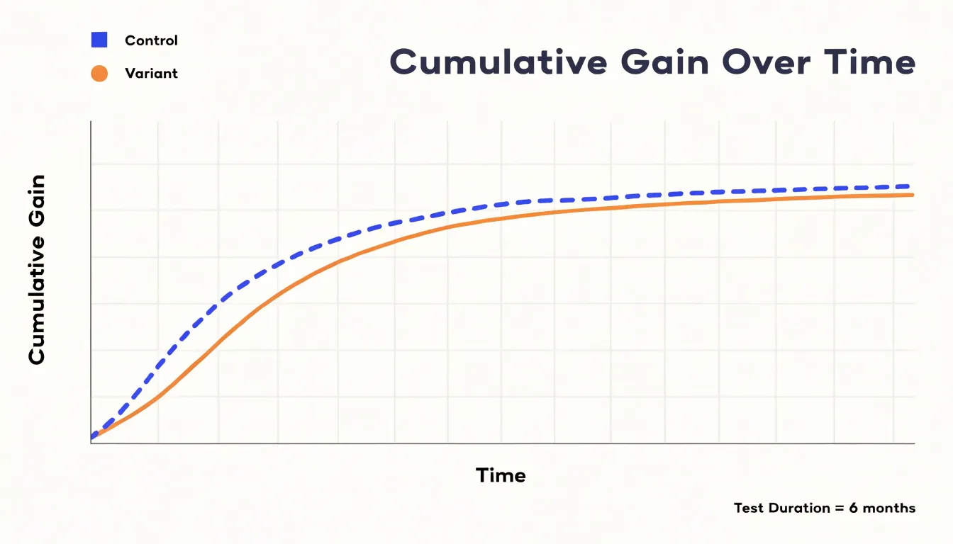
Lift charts complement cumulative gain by showing the relative improvement of a variant over the control, typically as a percentage. Early lift estimates can be volatile, but as the test progresses, the lift curve often smooths out, providing a clearer picture of the true effect size. Monitoring these charts helps analysts decide when to stop a test: once the cumulative gain and lift curves have converged to a stable pattern, additional data is unlikely to change the conclusion. This visual convergence also demonstrates to stakeholders how the evidence builds over time and highlights the point at which the data becomes trustworthy, offering a dynamic view of convergence that single-point metrics cannot provide.
Statistical Significance Charts
Statistical significance charts give teams a fast, visual way to judge whether an A/B test produced a genuine effect or merely a fluctuation that would have appeared on its own. At the center of these charts is the p-value, the probability of seeing an observed difference, or one more extreme, if no real difference exists between the two variants. Rather than asking readers to interpret a bare number, a significance chart plots the p-value over time or against the effect size, often alongside a horizontal reference line marking the chosen threshold, such as 0.05. When the plotted value drops below that line, the result crosses into conventional statistical significance, and the chart makes that crossing visible at a glance.
Some significance charts also pair p-value tracking with the confidence intervals described earlier, placing a vertical marker at zero to represent the no-difference baseline. If the entire interval sits above or below that zero line while the p-value stays below the threshold, both the direction and statistical reliability of the effect are clear in one view.
Visualizing these thresholds turns an abstract statistical question into a shared reference point. Product managers, designers, and analysts can look at the same plot and reach the same conclusion about whether a test has run long enough and produced a large enough effect to act on. This helps teams avoid the common pitfall of calling a winner too early based on an encouraging but unstable early spike, supporting more disciplined decisions about when to ship, iterate, or abandon a change.
Box Plots
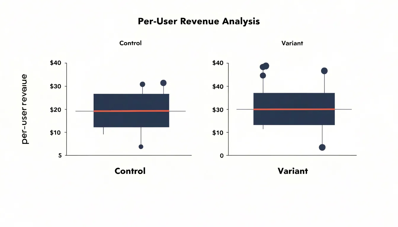
Box plots offer a compact visual summary of how revenue and spending are distributed across individual users in each test group. Rather than reducing a continuous metric to a single average, a box-and-whisker diagram displays the full shape of the data at a glance. The central box spans the interquartile range, from the 25th to the 75th percentile, showing where the middle half of users fall. The line inside the box marks the median spend, giving a robust measure of typical behavior that resists distortion from unusually large purchases. The whiskers extend outward to capture the rest of the distribution up to a defined boundary, often 1.5 times the interquartile range.
This structure is especially valuable for revenue metrics, which tend to be heavily skewed. A small number of high-value customers can pull the mean far above what most users actually spend, making averages misleading. The median and quartiles shown in a box plot keep the focus on the center of the distribution, so comparisons between the control and variant groups rest on a clearer picture of typical user behavior. Placing two box plots side by side makes differences in median spend, spread, and overall shape immediately visible.
Outliers are another key benefit. Points plotted beyond the whiskers flag individual users or transactions that sit far from the rest of the group. These extreme values deserve attention during analysis, since a handful of large purchases can influence the mean and the variance even when the median stays stable. A box plot surfaces these cases without hiding them inside an aggregate figure, letting analysts decide whether to investigate, segment, or treat them separately.
Funnel Charts
A funnel chart visualizes the sequential stages of a multi-step conversion process, such as a checkout flow or signup sequence, with each stage represented as a horizontal bar whose width is proportional to the number of users who reach it. This layout makes the progressive narrowing of the user base immediately apparent, highlighting exactly where drop-off occurs.
In an A/B test, funnel charts for each variant can be placed side by side, allowing you to compare the width of each stage between the control and the treatment. The difference in bar widths at a given stage reveals whether the variant improved or worsened progression at that specific step. For instance, if the variant shows a wider bar at the ‘add to cart’ stage but a narrower bar at ‘payment’, it indicates that the change encouraged more users to add items but created friction during payment. By pinpointing these stage-level differences, funnel charts help you isolate the impact of your changes, rather than relying on an aggregate conversion rate that can mask divergent effects across the funnel.
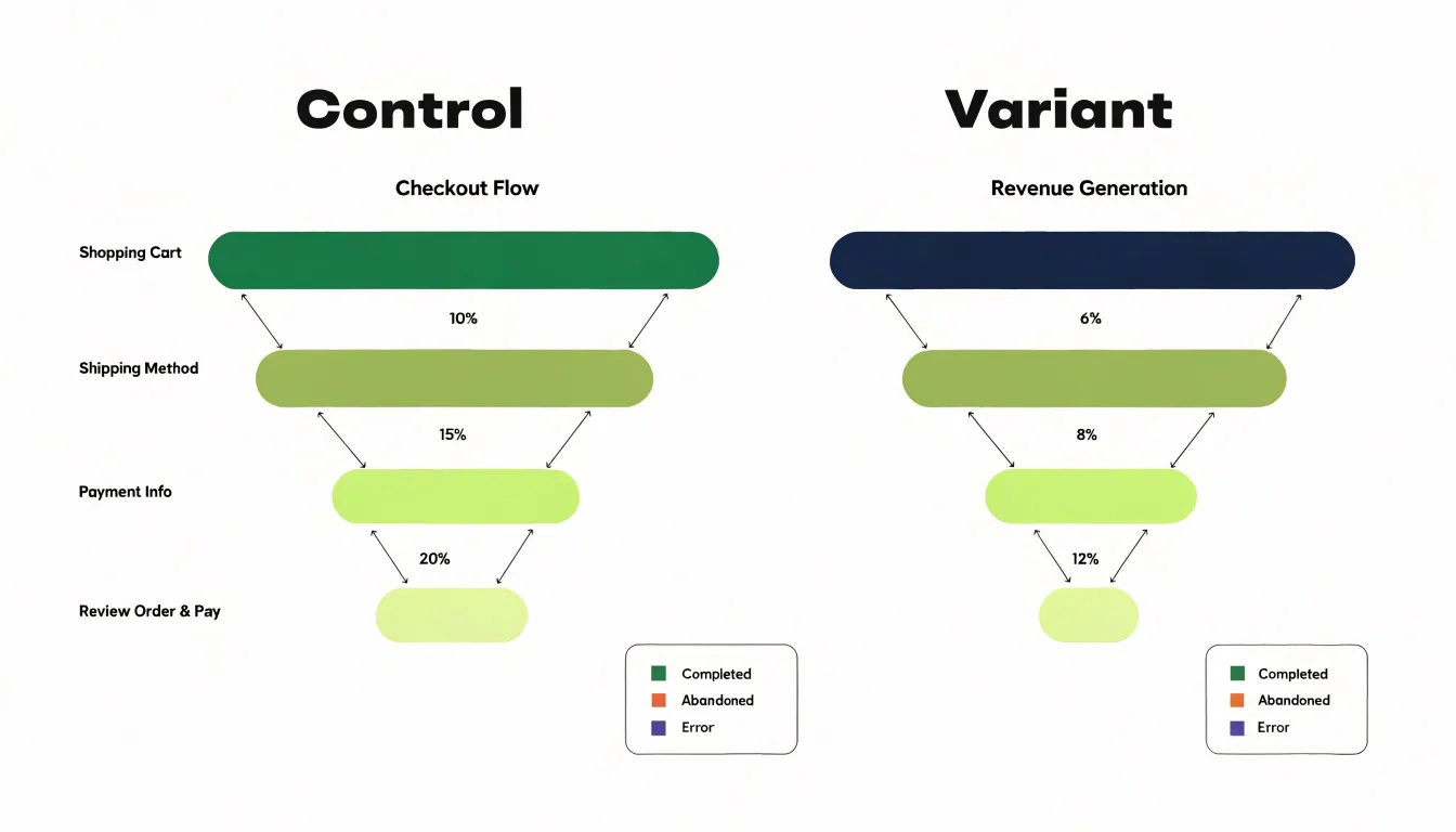
Moreover, funnel charts can display drop-off rates between stages, often as annotations or as separate segments, making it easy to identify the weakest link in the process. This stage-level insight is particularly valuable for prioritizing improvements: if the variant improves an early stage but harms a later one, you might decide to iterate on the later stage before rolling out the change. Because the visual metaphor of a funnel is intuitive, it immediately conveys to stakeholders where users are lost and helps direct optimization efforts to the parts of the user journey where they can have the greatest impact.
Sample Size Charts
Sample size charts serve as a critical checkpoint in the lifecycle of any A/B test, addressing one of the most common and costly mistakes in experimentation: making decisions before the data can support them. These charts track two values side by side over time, the required sample size calculated during test planning and the actual number of visitors or conversions accumulated so far. Presenting both on a single timeline gives researchers a clear visual answer to a simple but essential question: is this test finished, or does it still need time to run?
The required sample size is derived from the statistical parameters set before the test begins, including the baseline conversion rate, the minimum detectable effect the team wants to identify, the chosen significance level, and the desired statistical power. Together these inputs determine how many observations are needed for the test to reliably detect a real difference if one exists. The progress chart turns that number into a moving target the team can monitor, often plotted as a horizontal reference line that the accumulating actual sample size gradually approaches.
Without this visual tracking, teams frequently fall into the trap of checking results daily and stopping a test the moment a promising pattern appears. Early readings are dominated by noise, and a test paused at ten or twenty percent of its required sample can easily show a result that later reverses entirely. Progress charts counter this tendency by making the gap between required and actual sample size impossible to overlook.
These charts also help coordinate stakeholders around a shared expectation of timeline. When a product manager asks whether results are ready, the progress chart provides an objective answer grounded in statistical planning rather than impatience, keeping the experiment running until it reaches adequate power.
Time Series Line Graphs
Time series line graphs monitor daily performance in A/B tests by plotting conversion rates or other key metrics over the duration of the experiment. Displaying data points for each day reveals spikes, dips, and fluctuations that aggregate summaries obscure. For instance, a sudden surge in conversions on a particular day could indicate a promotional event, a mention in social media, or a technical glitch that temporarily boosted sign-ups. Similarly, a sharp decline might result from a server outage or an external factor like a holiday. When such anomalies appear, they can distort the overall test results if not properly accounted for.
Day-of-week effects are another critical consideration: user behavior often varies systematically—weekends may show lower engagement for B2B products, while consumer apps might see higher activity. A time series line graph makes these recurring weekly cycles visible, allowing teams to decide whether to adjust the test duration, segment the data by day type, or use statistical methods to control for day-of-week variability.
Moreover, the graph helps distinguish between random noise and meaningful trends. A gradual upward slope in one variant might suggest a genuine improvement, while erratic fluctuations could indicate instability. In practice, plotting daily conversion rates for both control and treatment groups on the same graph enables direct comparison. If one variant shows a spike that the other does not, it may point to an external event affecting only that group, such as a marketing campaign targeting a specific segment. Continuously monitoring the time series helps teams make informed decisions about when to pause, extend, or analyze the test further.
Heatmaps
Heatmaps translate raw interaction data into a visual layer that sits directly on top of the page being tested, so the differences between control and variant become immediately apparent. Click maps aggregate every tap, click, and in some tools every rage click into color-coded zones, with warmer tones marking the elements that attract the most attention. When you place the control and variant heatmaps side by side, shifts in where users click tell you whether a design change redirected focus toward the intended call to action or pulled it away toward secondary elements. Scroll maps work on a different axis, showing how far down the page visitors travel before they stop. A variant that keeps users engaged deeper into the page is strong evidence that the new layout, copy, or imagery is holding attention, while a heatmap that fades quickly reveals content that goes unseen.
The real value emerges when you layer the two views together. A button that glows red in the click map but sits inside a region where the scroll map has already gone cold points to a targeting or placement problem that conversion metrics alone would not explain. Comparing the two versions also surfaces engagement patterns that aggregate numbers flatten out, such as dead zones that appear only in the variant, or clusters of clicks on elements that look interactive but are not. These signals help you interpret why a test produced the result it did, giving designers and copywriters concrete, page-level feedback for the next iteration. Reading a heatmap takes a little practice, since color intensity reflects volume rather than sentiment, so pair the visuals with session recordings and segment-level data before drawing firm conclusions.
Distribution Curves
Probability density curves provide a clear visual representation of how the results of each variation are distributed. When you plot the density curves for two test groups on the same axes, the area where they overlap reveals the degree of uncertainty in comparing their performance. A large overlap indicates that the results are similar and that it is difficult to confidently determine which variation is better. As the overlap decreases, the separation between the curves grows, suggesting a higher probability that one variation truly outperforms the other.
The shape of each curve reflects the variability in the data. A narrow, tall curve indicates that the estimated effect is precise, with most outcomes clustered closely around the mean. A wide, flat curve suggests greater uncertainty, with outcomes spread over a broader range. By examining both the location (mean) and the spread (variance) of the curves, you can assess the likelihood that one variation’s true performance exceeds the other’s.
To quantify this, you can calculate the area under the curve where one variation’s results are greater than the other’s. This area corresponds to the probability that the variation is superior. For example, if the curve for Variation B lies mostly to the right of Variation A’s curve, the area under B’s curve to the right of A’s mean gives an estimate of the probability that B outperforms A. Instead of reporting only a p-value, showing the curves and highlighting the overlapping region makes uncertainty tangible, clarifying whether the data strongly favors one variation or whether more testing is needed.
Cohort Analysis Grids
Cohort analysis grids organize users into groups based on the period in which they first converted, then track each group’s behavior across subsequent periods. A typical grid places cohorts as rows, with time periods as columns, so that each cell shows the share of that cohort still active, still purchasing, or still subscribing at that point. Color-coded as a retention heatmap, the grid turns a dense table of percentages into a visual pattern where strong cohorts glow and weak ones fade. This makes it easy to see whether a lift in initial conversion produces users who stick around or merely users who arrive and leave.
For A/B test results, this matters because a higher conversion rate can hide a retention problem. A variant that doubles sign-ups may also attract users with weaker intent, so twelve weeks later its retention curve may sit below the control’s. The cohort grid surfaces that divergence by aligning the two arms side by side, letting you compare the same cohort age against the same cohort age. You can follow a single cohort row across columns to watch decay, compare cells diagonally to see whether newer cohorts are improving, or read down a column to judge how each test arm performs at a fixed point in the customer lifecycle.
Lifetime value calculations build naturally on the same structure. Multiplying retention rates by average revenue per active user across periods gives the cumulative value of each cohort, and charting those totals against the control shows whether the test’s gains hold. The grid also supports segment drill-downs, revealing whether retention differences concentrate in particular acquisition channels or plan tiers. Retention heatmaps reward patience, since the most convincing signals emerge several periods out, but they answer the question every conversion-focused test ultimately raises: did the lift last?
Scatter Plots
Scatter plots become valuable when an experiment tracks more than one continuous outcome and the team needs to see how those outcomes move together. Plotting two variables on the horizontal and vertical axes, with each point representing a unit of analysis such as a visitor segment, cohort, or test variant average, turns a pair of separate summaries into a single picture of the relationship between them. In an A/B test context, this visual layering makes it possible to compare variants across several metrics at once and to spot patterns that univariate summaries would obscure.
The most common use case is surfacing trade-offs. A variant might lift conversion rate while pushing average order value downward, so that the two effects pull revenue in opposite directions. On a scatter plot where conversion rate sits on one axis and average order value on the other, that tension appears as points clustered in different quadrants: a variant that converts more but sells smaller baskets lands far to one side and lower on the other. Viewing the variants as distinct point clouds instead of single numbers lets stakeholders see the spread within each group and judge whether the apparent trade-off is consistent or driven by a few extreme observations.
Scatter plots also support exploration of secondary metrics and guardrail measures. Plotting revenue per visitor against session duration, or engagement against refund rate, helps teams check whether a conversion gain coincides with a cost elsewhere in the funnel. Adding a trend line or confidence region around each variant’s points indicates the direction and strength of the association. The main requirement is that both axes represent genuinely continuous quantities and that points are labeled clearly by variant.
Segmented Bar Charts
Segmented bar charts—applying the grouped bar layout introduced earlier to specific user cohorts—reveal how different user groups respond to A/B test variants. By breaking down overall performance metrics such as conversion rate or click-through rate by demographic or traffic source, you can see whether a variant’s success is uniform or driven by a particular segment. For example, a new checkout flow might show a 5% overall lift, but a segmented bar chart could reveal that the lift is concentrated among returning visitors while new visitors actually experience a decline. This granular view helps you avoid misleading conclusions from aggregate data.
To create a segmented bar chart, group your users by relevant segments—such as age, gender, device type, or acquisition channel—and plot the performance metric for each variant side by side within each segment. This comparison makes it easy to spot segments where one variant clearly outperforms another, highlighting opportunities for personalization or targeted improvements.
Interpreting the chart requires attention to sample sizes within each segment. Small segments may produce noisy results, so consider whether differences are statistically significant, and be cautious about drawing causal inferences from demographic correlations. Used carefully, segmented bar charts move analysis beyond a one-size-fits-all conclusion and inform optimizations that resonate with specific groups.
Executive Summary Dashboards
An executive summary dashboard condenses the essential outcomes of an A/B testing program into a single, coherent view designed for leadership consumption. Decision makers rarely have time to inspect individual test results, segment breakdowns, or the full statistical detail behind each experiment. What they need is a clear answer to a straightforward question: what has testing delivered for the business, and where should attention go next? Aggregating key charts into one dashboard answers that question immediately, replacing scattered reports and ad hoc requests with a reliable, repeatable summary.
The structure of such a dashboard typically centers on a handful of high-level metrics. Cumulative lift in conversion rate or revenue per visitor, the number of tests concluded during the period, the share of tests producing statistically significant gains, and an estimated return on investment all belong at the top. Supporting visuals, such as a running trend line of aggregate lift or a compact bar chart of wins by business area, give context without demanding deep analysis. Each chart should be readable at a glance and consistent from one reporting cycle to the next, so leaders can track progress over time rather than reinterpreting a new format every month.
The practical value of this aggregation lies in speed and alignment. When leadership can see the program’s contribution in familiar business terms, conversations shift from questioning whether testing is worthwhile to deciding which opportunities deserve more investment. Dashboards also create a shared reference point across teams, reducing the risk of conflicting narratives about performance and keeping the testing program visible, funded, and connected to strategic priorities.
Frequently Asked Questions
What chart can compare conversion rates between A/B test variants?
Bar charts offer a direct way to compare conversion rates between a baseline control group and one or more test variants, with each bar’s height corresponding to its conversion rate. Grouped bar charts extend this by placing bars side by side within each group to compare multiple variants or segments against the control.
How do confidence interval plots help interpret A/B test results?
Confidence interval plots surround the point estimate of lift with a visual range reflecting how much that estimate could reasonably vary, often based on a 95 percent confidence level. They help readers judge whether the observed winner is clearly separated from zero or whether the interval straddles it.
What do cumulative gain graphs show during an A/B test?
Cumulative gain graphs track the running total of conversions or other key metrics for each variant throughout the test, plotting the cumulative sum against time or sample size. When the curves flatten and maintain a steady separation, it suggests the observed effect is stable and likely to persist.
How can funnel charts help analyze A/B test results?
Funnel charts visualize the sequential stages of a multi-step conversion process, with each stage’s bar width proportional to the number of users who reach it. Placing funnel charts for each variant side by side shows whether a variant improved or worsened progression at a specific step.
Why are sample size charts important in A/B testing?
Sample size charts track the required sample size calculated during test planning alongside the actual number of visitors or conversions accumulated so far. They help teams avoid stopping a test too early based on early readings that are dominated by noise.
What can heatmaps reveal when comparing A/B test variants?
Heatmaps overlay interaction data on the page, with click maps showing where users click and scroll maps showing how far down the page visitors travel. Placing control and variant heatmaps side by side reveals shifts in where users click or how deeply they engage, which can help explain why a test produced its result. The article cautions that color intensity reflects volume rather than sentiment, so pair the visuals with session recordings and segment-level data before drawing firm conclusions.
Tony Astor
Tony writes about data visualization and the tools people use to build charts and dashboards. More about Data Illustrator