Beeswarm vs Strip Plot: Showing Individual Data Points
 By Tony Astor ·

Beeswarm vs Strip Plot
A beeswarm plot and a strip plot both show every observation as an individual point, but differ in how they handle overlap. A strip plot places points at fixed or jittered positions, keeping values exact but letting dense points overlap; a beeswarm plot shifts points sideways only enough to avoid collisions, preserving exact values while revealing density.
Table of Contents
Strip Plot
A strip plot represents each observation as a single point positioned along a numerical axis. In its most basic form, the horizontal or vertical position of a dot encodes the measured value, and nothing else is added on top: no boxes, no summaries, no smoothing. Every record in the dataset becomes one visible mark, offering a direct, unfiltered view of the raw measurements. If a sample contains forty observations, the plot shows forty points, each sitting at its exact recorded value.
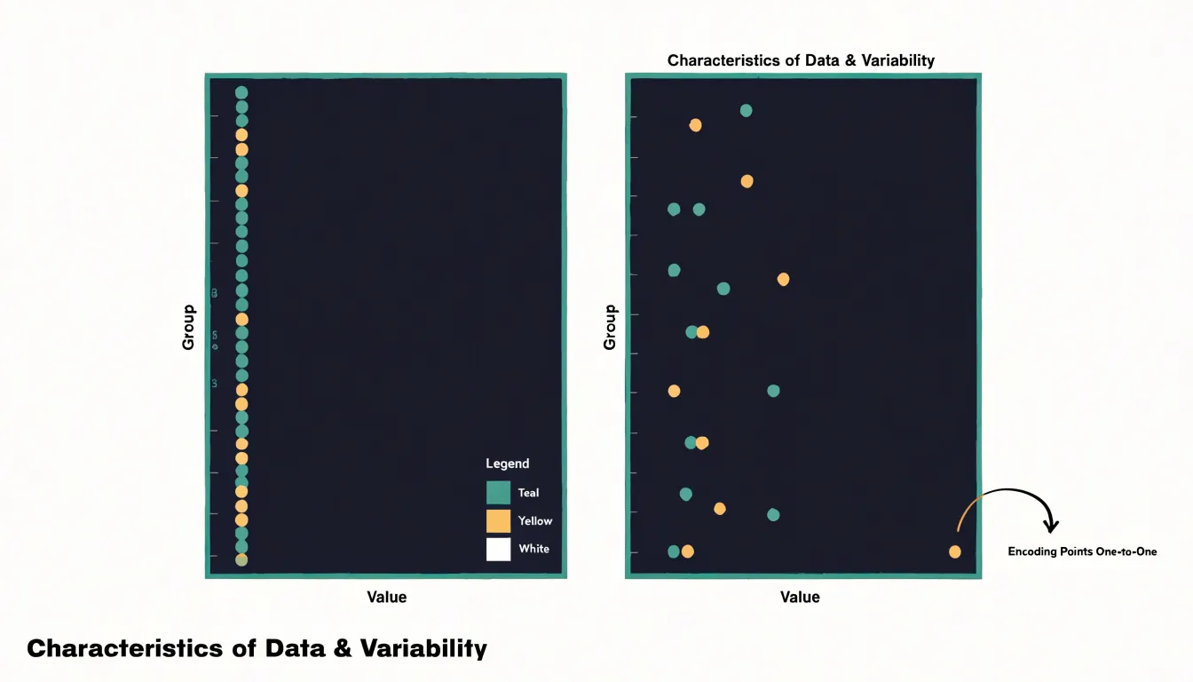
This one-to-one mapping makes strip plots well suited to simple categorical comparisons. A common layout places several categories side by side along a discrete axis, with each group’s points arranged in a vertical column at that category’s position. The reader can scan across the categories and compare where the values cluster, how wide they spread, and whether any points sit apart from the rest. The structure stays minimal: a numerical axis, a categorical axis, and points.
Strip plots work best when the data density is low. With a modest number of observations per category, the points remain individually distinguishable, and the chart communicates the full distribution without any intermediate statistics. The reader sees the actual values rather than a summary derived from them, which supports careful inspection of the sample.
Because every point occupies a precise location, strip plots also make specific values easy to locate and discuss. An unusually high or low observation appears as a solitary dot at the edge of its column, drawing attention naturally. When observations share identical or near-identical values, the points overlap, which signals repeated measurements at that value. For simple, low-density categorical comparisons, this direct point-based encoding keeps the chart honest and easy to read.
Jitter
Jitter addresses the common problem of overplotting in strip plots, where multiple data points share the same or nearly the same value. When many observations fall into the same category and have similar numeric values, they are plotted at the same position, causing points to overlap and obscure one another. Jitter mitigates this by adding a small amount of random noise or offset to the coordinates of each point, typically along the categorical axis. This spreads the points out horizontally, reducing overlap and revealing the underlying structure of the data.
The added noise is usually drawn from a uniform or normal distribution with a small scale relative to the spacing between categories. The amount of jitter must be chosen carefully: too little jitter fails to resolve overlaps, while too much jitter can distort the perception of the categorical grouping, making points appear to belong to adjacent categories. A common default is to use a jitter width that is a fraction of the distance between categories, often around 0.1 to 0.3 of the category width.
Jitter is particularly useful when the dataset is large or when the numeric variable takes on discrete values, leading to many ties. Spreading points horizontally provides a clearer view of the number of observations at each value and the overall shape of the distribution. However, because it introduces artificial variation, the jittered positions should not be interpreted as precise numeric values. Analysts often combine jitter with transparency (alpha blending) to further reduce visual clutter, allowing overlapping points to be distinguished by darker regions where many points coincide.
Beeswarm Plot
When many observations share the same or nearly the same value on one axis, their markers land on top of one another, concealing how many points are truly present. The beeswarm layout addresses this by allowing points to shift sideways within a narrow band, displacing each marker just enough to clear its neighbors while leaving its original value untouched. The result is a cloud of points that swells where observations cluster and thins where they are sparse, so density becomes visible directly through the shape of the swarm.
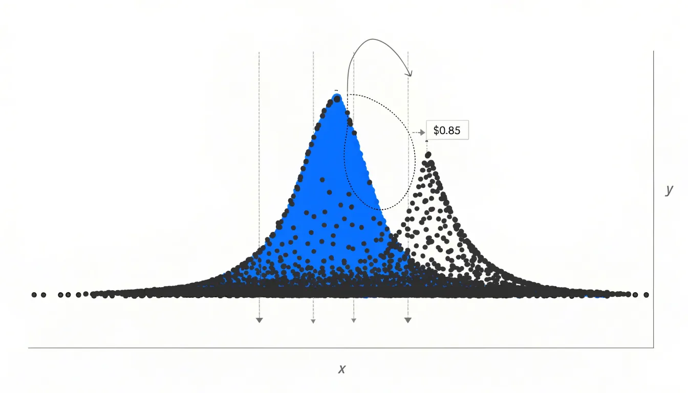
The mechanics rely on deterministic algorithms, meaning the same input data always produces the same layout. A typical procedure sorts the points by their value on the primary axis, then places them one at a time. Each point is offset along the perpendicular axis in small increments, alternating to one side and then the other, until it finds a position that does not overlap any previously placed marker. Some implementations use a fixed collision radius; others use variable radii proportional to marker size. More refined versions choose the smallest displacement that avoids collisions, which keeps the swarm tight and symmetric.
Because the displacement happens along the perpendicular axis, the vertical position of every point, or horizontal in a horizontal orientation, remains exactly equal to its data value. The beeswarm adds a second dimension of visual information without altering the first. Readers can therefore read individual observations precisely while also perceiving the frequency distribution as a whole. This combination of exact value preservation and density revelation makes the beeswarm a natural fit for datasets with repeated or rounded measurements, where a plain scatterplot would collapse into indistinguishable stacks.
Beeswarm vs Strip Plot
When laying out a beeswarm chart and a strip plot side by side, the mechanics of placement reveal meaningful differences. A strip plot positions points along a categorical axis, typically jittering them with random or evenly spaced offsets within a band. A beeswarm chart, by contrast, arranges points in a swarm-like formation where each marker is placed as close to the central axis as possible without colliding with its neighbors, producing a tightly packed, symmetrical shape that resembles a swarm of bees.
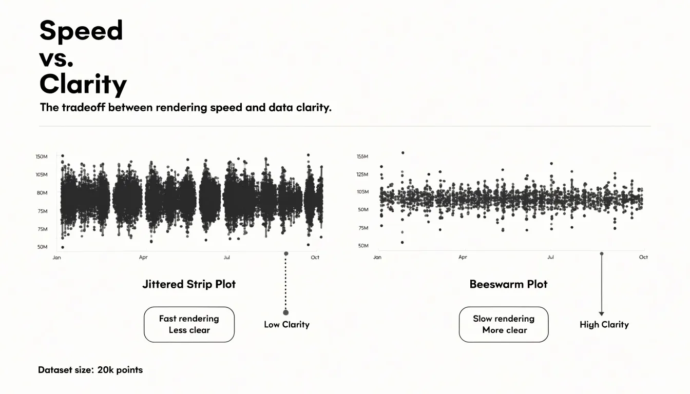
Point alignment differs accordingly. In a strip plot, points often align along fixed grid positions or random jitter offsets, which can create clumps and gaps. A beeswarm chart enforces a collision-avoidance rule, so points shift to maintain spacing, yielding a more organic and evenly distributed layout. This alignment affects how density is perceived: strip plots can obscure density when points overlap heavily, while beeswarm charts preserve individual points and make local density visible.
Computational complexity is a practical differentiator. Strip plots require minimal computation, as jitter offsets are generated with a simple random or deterministic function. Beeswarm charts require iterative collision detection, often using force-based simulations or greedy placement algorithms, which increases processing time and memory use, especially with large datasets. For interactive or real-time visualizations, this complexity matters.
Visual clarity follows from these mechanics. Strip plots are easy to read and fast to render, but overlapping points can hide structure. Beeswarm charts avoid overlap, making each observation distinguishable and revealing distribution shape, though they can become dense and visually busy with thousands of points. The layout also affects how outliers and clusters appear, with beeswarm charts offering a clearer sense of local concentration.
Small Data Sets
Strip plots excel in the setting of small data sets, where each group contains fewer than roughly thirty observations. With so few points, a one-dimensional scatter along a categorical axis keeps every individual value visible, so the reader can trace each observation back to its source without any intermediary summarization. This transparency matters because small samples are sensitive to individual values. A single unusual measurement can shift a group mean or inflate a standard deviation, and hiding that point inside an aggregated shape obscures the information an analyst needs.
When a group holds only a handful of points, the mark for each observation stands on its own. There is no crowding, no overplotting, and no need for jitter to separate coincident values, because there are simply too few values for marks to collide. Readers can count the observations in each group directly from the chart and compare group sizes at a glance. This direct correspondence between data and display keeps the cognitive load low: the eye moves along the categorical axis, registers the position of each dot, and forms a comparison without needing to decode density, bandwidth, or distributional shape.
Strip plots also avoid the assumptions that come with smoothed representations. A histogram or density curve built from a dozen points imposes binning or kernel choices that can misrepresent the underlying sample, producing shapes that suggest structure the data cannot support. A strip plot makes no such commitments. It presents the raw values in their natural positions and lets the reader draw conclusions at the level of individual observations, making it a dependable choice whenever group sizes stay below the thirty-point threshold.
Dense Data
Beeswarm plots are particularly effective for dense datasets, where hundreds of observations would otherwise overlap in a standard or jittered strip plot. By systematically shifting points sideways only as much as needed to prevent collisions, the beeswarm layout expands outward as density increases, accommodating hundreds of points without sacrificing clarity or altering exact values on the primary axis.
For datasets with a few hundred points, the beeswarm layout remains readable, though at very high densities (thousands of points), the swarm may become overly wide and require careful scaling or alternative approaches. Nevertheless, for typical exploratory data analysis with moderate to large samples, beeswarm plots offer a graceful solution to overplotting, balancing individual point visibility with an honest representation of data density. This makes them especially useful in fields like biology, where researchers often need to display individual observations alongside summary statistics, or in any context where the fine-grained structure of the data matters.
Distribution Patterns
Because both the beeswarm and the strip plot preserve individual data points as visible marks, a viewer can trace the shape of the underlying distribution directly from the canvas. In a strip plot, clusters, gaps, and long tails appear as literal concentrations or absences of dots along the primary axis. When the data are bimodal, two distinct bands of points emerge with a visible empty corridor between them; when the data are skewed, the dots thin out gradually toward one end of the axis. Because nothing has been collapsed into a single mean or median, the viewer reads the distribution shape from the density of marks rather than inferring it from a table of summary values.
The beeswarm plot retains this virtue while adding horizontal spread to signal how crowded a region of the distribution is: dense central regions fan out into wider swarms, while sparse tail regions contain only a few loosely spaced dots. This retention of raw detail supports the recognition of features that summary statistics routinely obscure. A mean and standard deviation can describe a symmetric bell-shaped dataset adequately, yet they describe a bimodal dataset poorly, since the two modes may average into a value that few or no observations actually take. By keeping every point visible, both plot types let viewers notice secondary peaks, isolated outliers, and abrupt changes in density without needing to consult a separate histogram or density curve.
Categorical Groups
When comparing ratings across categories, the arrangement of categorical groups along the secondary axis plays a critical role in how effectively viewers can draw cross-group comparisons. Start by ordering categories based on a meaningful sequence: alphabetical order works for lookup tasks, but for analytical comparisons, sort categories by median rating, sample size, or another relevant metric. This ordering guides the eye toward trends and highlights extremes. If there is a natural hierarchy or grouping among categories, such as geographic regions or product tiers, group related categories together and separate groups with subtle spacing or dividers to reinforce structure.
For multiple categories, consider using small multiples: place each category in its own panel along the secondary axis, aligned vertically or horizontally. This approach prevents overcrowding and allows consistent scaling across panels, making it easier to compare distributions side by side. When many categories share a single axis, avoid excessive jitter that can obscure patterns; instead, use a hybrid approach that combines a strip plot for individual points with a beeswarm layout to reduce overlap while preserving the distribution’s shape.
Color and shape can encode category membership, but rely on position and alignment as primary cues. Ensure that the secondary axis labels are clear and consistently placed, using tick marks and grid lines to aid reading. If categories are nested (e.g., subcategories within main categories), use faceting or hierarchical labeling to maintain clarity. Finally, test the arrangement with a small audience to ensure that comparisons are intuitive and that no category is visually marginalized.
Overcrowding
Overcrowding is a common failure mode for both strip plots and beeswarm plots. In a strip plot, once dozens of points share nearly the same value, the plot collapses into a dense band where individual observations can no longer be distinguished. While a beeswarm plot mitigates this for small and moderate samples, its displacement has limits: when the local density of points exceeds the available space at a given position, the swarm algorithm must push points further out or begin stacking them, and the tidy appearance degrades into an irregular blob that misrepresents where the data actually concentrate.
The practical threshold is best judged by whether individual points remain identifiable. If you cannot tell how many observations sit at a particular value, or if the offset distance needed to separate points becomes larger than the scale of meaningful variation in the data, the plot has broken down. Very large samples, heavily discrete or rounded values, and datasets with extreme local clustering all accelerate this breakdown. In these situations the visual encoding of individual points stops carrying reliable information and starts creating visual noise.
At that point, switching to a box plot or a violin plot is the right move. Both summarize the distribution rather than displaying every observation, so they remain legible regardless of sample size. A box plot emphasizes the median, quartiles, and outliers, while a violin plot shows the estimated density shape, which is especially useful when the underlying distribution is multimodal. The transition preserves the reader’s ability to compare groups while avoiding the clutter that undermines interpretation.
Tools
A range of data visualization libraries support both strip plots and beeswarm plots, making it straightforward to generate either style from the same dataset:
- Python (Seaborn): Provides a high-level interface for strip plots through its
stripplotfunction and supports beeswarm-style plots viaswarmplot. These functions handle the underlying layout calculations, including jitter and collision avoidance, while allowing customization of colors, markers, and groupings. Seaborn integrates seamlessly with pandas DataFrames. - R (ggplot2 and base R):
ggplot2offersgeom_jitterfor strip plots andgeom_beeswarmfrom theggbeeswarmpackage for beeswarm plots, enabling layered customization and consistent syntax. Base R functions likestripchartprovide simple strip plot capabilities, and thebeeswarmpackage offers dedicated beeswarm functionality. - JavaScript (D3.js): Provides the low-level primitives needed to build both plot styles from scratch. Its force simulation module can be adapted to create beeswarm layouts by applying collision forces, while simple SVG circles positioned with jitter produce strip plots. D3.js affords complete control over rendering and interaction for web-based dashboards and custom visualizations.
- Other tools: Plotly (with strip and swarm modes) and Vega-Lite (which supports jitter but not native beeswarm) offer additional options.
When choosing a tool, consider the need for interactivity, integration with existing workflows, and the level of customization required. For quick exploratory analysis, Seaborn and ggplot2 are often sufficient; for production web applications, D3.js or Plotly may be preferable. Many of these libraries also allow exporting plots as static images or interactive HTML, facilitating sharing and publication.
Design Tips
Choosing point sizes and colors for readability begins with the density of the data itself. In a beeswarm plot, each marker needs to stay small enough that tightly packed neighbors remain distinct while large enough to register as a clear shape. A point diameter of roughly 4 to 8 pixels works well for most displays; when categories hold many observations, err toward the smaller end and let the arrangement carry the structure. For strip plots, where points overlap heavily, smaller markers paired with higher opacity help reveal clusters without turning dense regions into solid blocks. Opacity in the range of 0.5 to 0.8 is a practical starting place, and it should tighten as point count rises, since transparency lets overlapping observations accumulate visually into darker areas that signal concentration. A thin stroke is equally important: a one-pixel border in a shade slightly darker than the fill keeps individual points legible against a light background and separates them where they touch.
For color palettes, limit yourself to a small set of hues drawn from a perceptually uniform scale, assigning color to a meaningful category or a continuous variable rather than decorating the chart. Light, desaturated fills work best for single-series plots, while stronger hues suit comparisons across a few groups, provided adjacent colors remain distinguishable for viewers with color vision deficiencies. Test the final combination at the intended display size, checking that isolated points read clearly and that dense regions retain visible texture, then adjust opacity and stroke width together until both extremes hold up.
Hybrid Charts
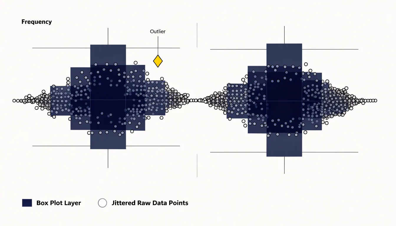
Hybrid charts combine a summarized statistical layer with a layer of raw data points, so that a single visualization communicates both the distribution’s key metrics and the individual observations that produced them. A common form places a box plot at the center of the figure, showing the median, the interquartile range, and any flagged outliers, while the raw points for each group are drawn alongside or over the box in a jittered arrangement. The box supplies the summary metrics at a glance, and the points reveal the sample size, the shape of the distribution, and any clustering or gaps that summary statistics alone would conceal.
Violin plots work in the same layered fashion. The violin outline shows a smoothed density estimate for each group, and the raw points can be overlaid inside the violin body or arranged next to it. This arrangement lets a reader see where observations concentrate and also inspect the individual values behind the smoothed curve. When the sample is small, the density estimate of a violin can be misleading, and the visible points make that limitation clear.
Layering raw data over summary graphics also improves transparency about outliers and sample size. A box plot flags an observation as an outlier through a rule based on quartiles, but the reader cannot see how many such points exist or how far they sit from the rest of the data. Adding the raw points exposes that information directly. Similarly, two groups with identical medians and interquartile ranges can look the same in a box plot even when one contains a dozen observations and the other contains several hundred; the point layer makes the difference obvious.
In these hybrid charts, points should be drawn with partial transparency and a small amount of horizontal jitter so that overlapping values remain readable. The summary layer should sit behind or beside the points rather than obscuring them, and the legend should make clear which visual element represents the summary and which represents the raw observations.
Outliers
Outliers deserve special attention in any point-based display because a single extreme value can reshape the reader’s impression of the entire dataset. In a strip plot, outliers sit within a column of points, and their distance from the main cluster makes them visible, though they can also stretch the axis and compress the rest of the distribution into an unreadable band. A beeswarm layout offers a partial remedy: by displacing points sideways, dense regions spread out while isolated values remain distinct, so a lone observation at the far end of a category reads as separate rather than as part of a crowded line.
Techniques for highlighting these extremes include:
- Color: Assign a contrasting fill color to points beyond a threshold, often defined using the interquartile range or a fixed number of standard deviations from the median.
- Annotations: Place a short label beside an anomalous point, or use a thin leader line connecting it to its category label, drawing the eye without requiring a separate legend.
- Size and shape: Render flagged points as larger diamonds while ordinary observations stay as small circles. Where several outliers share a category, a subtle halo or outline helps them stand out from overlapping neighbors.
- Interactivity: Reveal the exact value and identifying label of an outlier on hover while dimming the remainder of the plot.
Ensure that highlighting rules are documented in the caption, since readers will want to know what counts as extreme and whether thresholds were chosen before or after inspecting the data. Combined with a robust axis range or a broken scale, these cues let analysts spot anomalies quickly while preserving the overall shape of the distribution.
Decision Guide
When deciding between a strip plot, jittered strip plot, and beeswarm plot, start by counting the number of observations per category:
- Fewer than ~20 points per group: A simple strip plot works well, placing each data point at its exact value without overlap.
- 20 to 100 points per group: Overplotting becomes a concern. A jittered strip plot preserves the exact vertical position while reducing overlaps. Because jitter can obscure the precise x-value, it is best when the audience needs to see individual points rather than estimate exact counts.
- More than ~100 points per group: A beeswarm plot is often the better choice, avoiding overlap while keeping each point distinguishable and revealing density, provided there is enough horizontal space and the dataset is not so large that it becomes cluttered.
Beyond dataset size, consider your audience’s needs and the presentation medium. If the goal is to show raw data transparently—for example, in a scientific poster—a strip or jittered strip plot may be preferred because it does not imply a smoothed density. If the goal is to compare distributions across categories while maintaining point-level detail, a beeswarm plot offers a compact solution. Interactive dashboards can benefit from jittered plots with tooltips, while static reports often favor beeswarm plots for their clarity.
Overview
A dashboard-style summary provides a quick-reference matrix for deciding between beeswarm and strip plots across recommended use cases, strengths, and limitations:
- Beeswarm Plots
- Recommended use cases: Datasets with a moderate number of points (roughly 10 to 100 per category) where the goal is to reveal distribution shape, identify clusters, or spot outliers without overplotting.
- Strengths: Shows every individual observation while avoiding overlap; intuitive appeal for non-expert audiences; effective at highlighting local density patterns.
- Limitations: Reduced effectiveness with very large datasets (where points become too small or densely packed); potential distortion of the underlying distribution due to algorithmic point placement; risk of misinterpretation when points cluster in ways that suggest false gaps or peaks.
- Strip Plots
- Recommended use cases: Very small datasets (fewer than 10 points per category) where simplicity is paramount, or very large datasets (hundreds or thousands of points) where individual points are less important than overall density and where jittering can approximate a density estimate.
- Strengths: Simplicity, computational efficiency, and ease of implementation in most plotting libraries.
- Limitations: Overplotting with moderate sample sizes; arbitrary jitter that can obscure precise values; difficulty in comparing distributions across categories when points are spread horizontally.
Presenting this matrix as a table or a decision tree guides analysts based on sample size, the importance of individual points, and the need to compare distributions, helping them select and justify the appropriate visualization in reports or publications.
Frequently Asked Questions
What is a strip plot?
A strip plot represents each observation as a single point positioned along a numerical axis, with no boxes, summaries, or smoothing added. Every record in the dataset becomes one visible mark, making strip plots well suited to simple categorical comparisons and low-density data.
Why use jitter in a strip plot?
Jitter adds a small random offset, typically along the categorical axis, to reduce overplotting when multiple points share the same or nearly the same value. The amount must be chosen carefully, because too much jitter can distort the perception of categorical grouping.
How does a beeswarm plot keep points from overlapping?
A beeswarm plot uses deterministic algorithms to shift points sideways within a narrow band just enough to clear neighboring markers while leaving their original value untouched. This makes density visible through the shape of the swarm while preserving exact values on the primary axis.
When should I choose a beeswarm plot over a strip plot?
For more than roughly 100 points per group, a beeswarm plot is often the better choice because it avoids overlap while keeping each point distinguishable and revealing density. This assumes there is enough horizontal space and the dataset is not so large that it becomes cluttered.
What should I do if a strip plot or beeswarm plot becomes overcrowded?
When individual points are no longer identifiable, or the offset needed to separate points becomes larger than the scale of meaningful variation, switching to a box plot or violin plot is the right move. A box plot emphasizes the median, quartiles, and outliers, while a violin plot shows the estimated density shape.
Can strip plots and beeswarm plots show the shape of a distribution?
Yes. Because both plot types preserve individual data points as visible marks, viewers can trace clusters, gaps, long tails, bimodal bands, and skew directly from the density of marks. A beeswarm plot also adds horizontal spread to signal how crowded a region of the distribution is.
Tony Astor
Tony writes about data visualization and the tools people use to build charts and dashboards. More about Data Illustrator