Beeswarm Plot: Distributions Without Overlapping Points
 By Tony Astor ·

Beeswarm Plot
A beeswarm plot is a one-dimensional scatter plot that places one marker per observation along a value axis and offsets overlapping points perpendicular to that axis, so every data point stays visible. The swarm’s width shows local density, revealing clusters, gaps, multimodality, and outliers that bar charts, box plots, and histograms hide.
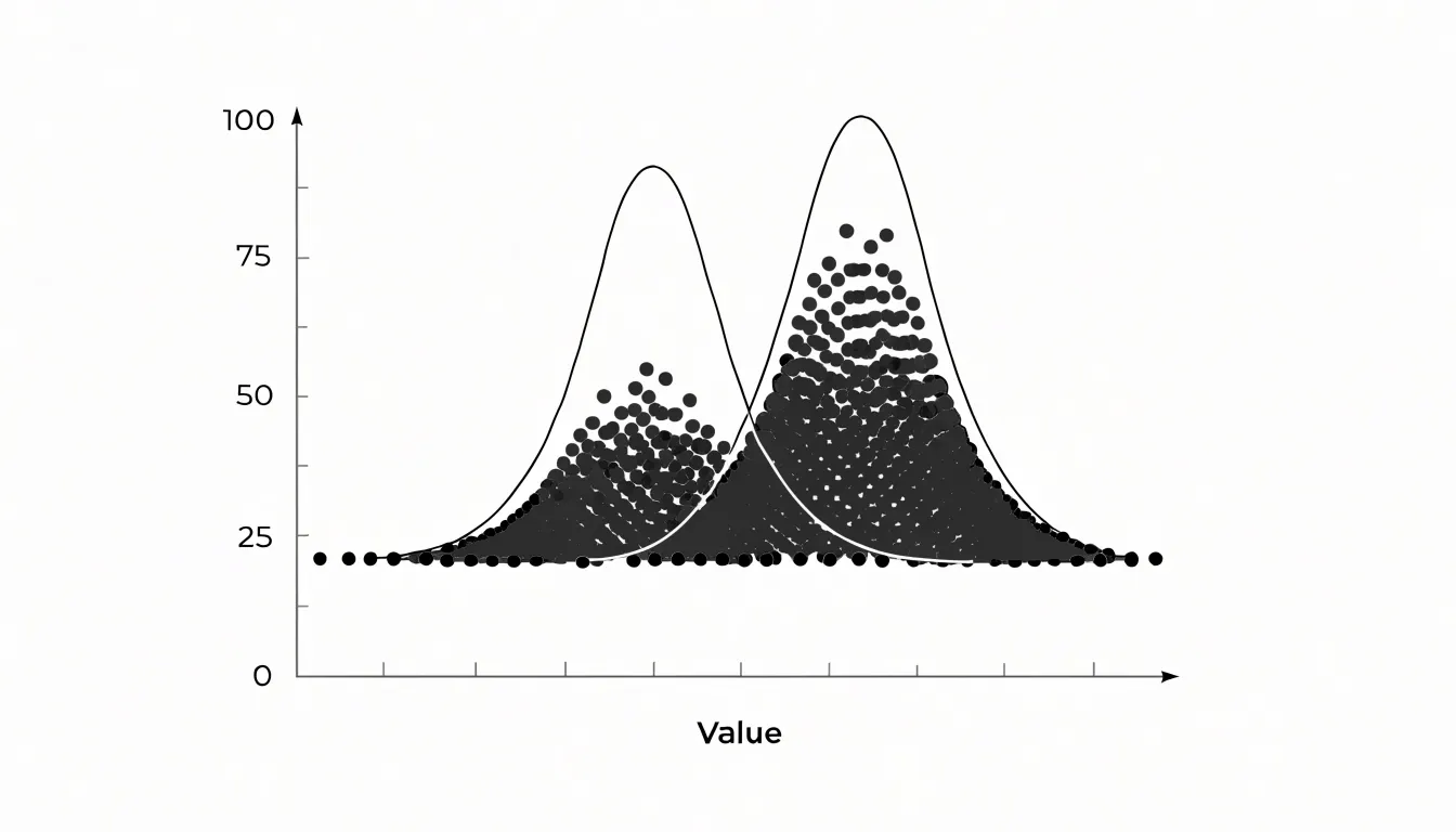
Table of Contents
- Beeswarm Plot
- Beeswarm vs. Box Plot
- Beeswarm vs. Bar Chart
- Beeswarm vs. Violin Plot
- Swarm Layout Mechanics
- Reading Individual Points
- When to Use Beeswarm Plots
- Handling Large Datasets
- Point Radius
- Color Coding
- Python Beeswarm Plots
- R Beeswarm Plots
- Avoiding Common Mistakes
- Real World Applications
- Dashboard Overview
Beeswarm Plot
A beeswarm plot begins with the same premise as a strip plot: every observation in a dataset receives its own mark, placed along a single axis at the position of its measured value. The distinguishing feature lies in how the plot handles collisions. When many observations share similar or identical values, a simple strip plot stacks them on top of one another, hiding the density and frequency of the underlying data. The beeswarm algorithm resolves this by displacing points perpendicular to the value axis so that each marker remains individually visible.
The positioning typically proceeds value by value. Points are sorted along the primary axis, then placed one at a time. For each new point, the algorithm searches outward from the axis in both perpendicular directions, testing candidate positions against the markers already placed. A location is accepted only when the new point does not overlap any existing marker. The search stops at the nearest such gap, keeping each point as close to the central axis as geometry allows. The result is a compact, symmetrical arrangement that resembles a swarm, with dense clusters bulging outward and sparse regions staying close to the axis.
Because every observation retains its own visible marker, the plot preserves the full sample. Readers can count points, spot outliers, and see multimodal distributions without the smoothing or binning associated with histograms or density curves. The width of the swarm at any value reflects local density, so the overall silhouette communicates distribution shape while individual dots remain intact. This makes beeswarm plots especially useful for modest to moderate sample sizes, where each observation carries information and an aggregate summary would discard meaningful detail.
Beeswarm vs. Box Plot
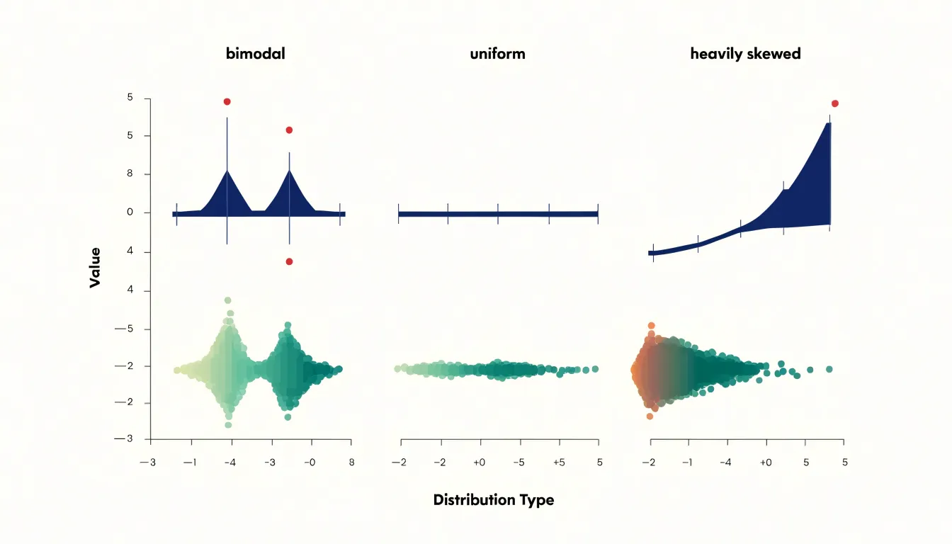
A box plot condenses a distribution into five summary statistics: minimum, first quartile, median, third quartile, and maximum, often with whiskers extending to a defined multiple of the interquartile range. This compression makes box plots compact and easy to compare across many categories side by side, but the abstraction hides the shape of the underlying data. A bimodal distribution, a uniform spread, and a heavily skewed sample can all produce similar-looking boxes, and clusters of concentrated values are invisible.
By drawing one marker per observation, a beeswarm plot reveals where observations cluster, where gaps appear, whether the distribution is unimodal or multimodal, and whether outliers form an isolated group or connect smoothly to the main mass. Reading a beeswarm plot at a glance gives both the individual data points and the overall density profile simultaneously.
Box plots remain valuable when the number of groups is large, when the dataset is too big to render individual points, or when precise quartile comparisons are the analytical focus. Beeswarm plots become preferable when sample sizes are moderate, when distribution shape matters to the question at hand, and when the audience needs to see exact observations rather than summary statistics. A quick screening across dozens of categories favors box plots, while a detailed examination of a handful of groups rewards the granular display of a beeswarm. Combining the two views in one figure, with a box or violin overlaid on the swarm, can capture summary metrics and point-level detail together, letting readers move between the compressed and the granular picture of the same distribution.
Beeswarm vs. Bar Chart
Traditional bar charts summarize data using a single value, typically the mean or median, which collapses the full distribution into one height. This aggregation hides the spread of the data, the presence of outliers, and the shape of the distribution.
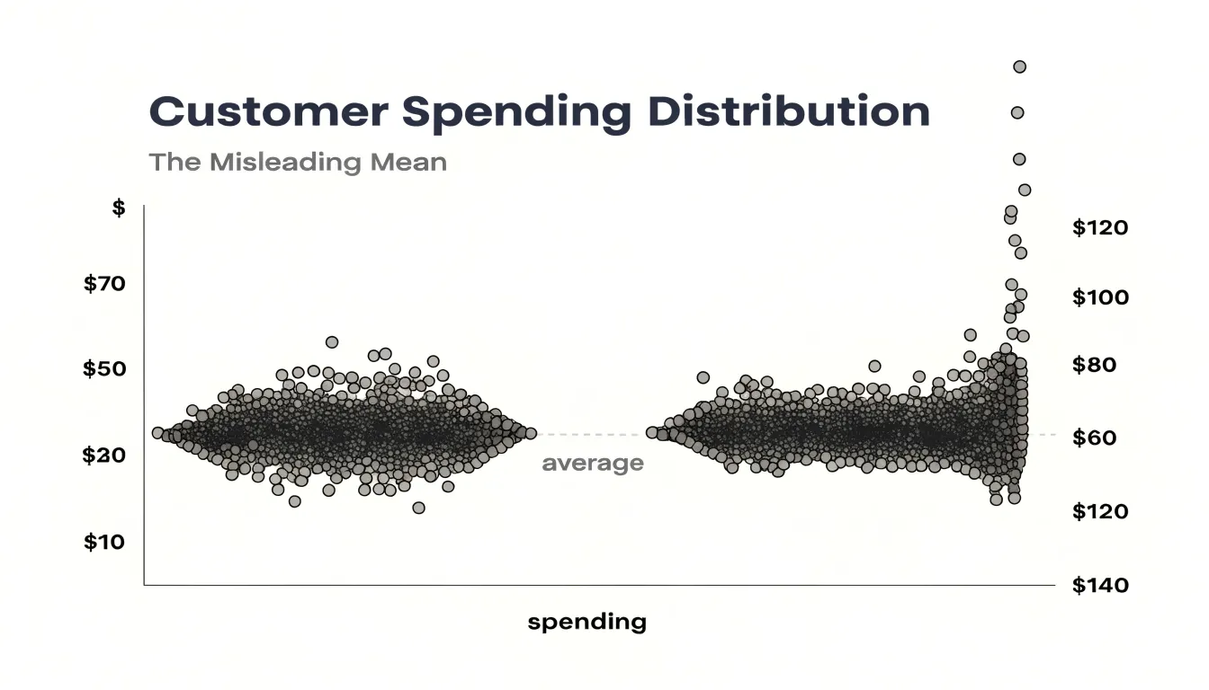
When data is bimodal or contains distinct clusters, a bar chart shows only an average that may not represent any actual group. For example, a bar chart of customer spending might show an average of $50, while the underlying data consists of two groups: budget shoppers spending around $20 and premium shoppers spending around $80. The average of $50 misrepresents both groups and obscures the bimodal pattern. Similarly, hidden clusters—such as a small segment of high-value customers—are invisible in a bar chart because their values are averaged away.
In the customer spending example, a beeswarm plot clearly shows two distinct clusters—one around $20 and another around $80—along with any small group of customers spending significantly more than the rest. Preserving individual points exposes multiple modes and patterns that single summary statistics obscure.
Beeswarm vs. Violin Plot
Violin plots and beeswarm plots both visualize distributions, yet they encode information differently. A violin plot uses kernel density estimation to produce a smooth, mirrored shape that conveys the probability density of values across a range. The width of the violin at any point indicates how many observations are concentrated there, offering an immediate sense of whether the distribution is unimodal, bimodal, or skewed. However, the raw observations are aggregated into a continuous curve, and the exact values are obscured.
In contrast, a beeswarm plot’s point-level display allows viewers to see actual data values, sample size, and precise locations without the smoothing artifacts of kernel density estimation, making it easier to spot gaps, ties, or unusual observations. While violin plots excel at summarizing overall density and comparing multiple groups through mirrored shapes, beeswarm plots combine density cues with the authenticity of individual values. For a quick impression of distribution shape and density, violin plots are efficient; for detailed inspection of specific records and patterns, beeswarm plots provide greater fidelity. In practice, the two can be layered so the beeswarm reveals the raw data structure that the violin summarizes.
Swarm Layout Mechanics
Swarm layout mechanics keep every encoded value exact while resolving collisions. When the quantitative variable sits on the Y-axis, each observation occupies a fixed vertical position determined by its measured quantity, and horizontal displacement is used purely to resolve overlap, carrying no data meaning of its own. The layout engine treats each point’s vertical coordinate as immovable and searches only along the horizontal line at that height for a free slot. A common implementation sorts points by their vertical value and processes them in order, attempting to place each new point at the center and then testing candidate offsets of increasing magnitude, alternating left and right, until a position is found that clears every previously placed marker by at least the marker radius plus a small buffer. This greedy collision test is cheap to compute and produces a symmetric, teardrop-like profile.
Symmetry deserves care, since naive left-right alternation can drift if the collision checks are uneven. Many libraries run a two-sided pass, computing free horizontal intervals on each side of the anchor and choosing the nearer valid slot, which balances the swarm visually.
Performance matters at scale. Efficient implementations maintain a structure of occupied intervals rather than testing every prior point, reducing the cost from quadratic toward linear in most practical datasets. Some variants bin nearby y-values into shared rows to limit expansion, at the cost of slight vertical jitter that must be disclosed. Throughout, the guiding constraint remains constant: the packing algorithm may translate points perpendicular to the value axis, but it never edits their quantitative position.
Reading Individual Points
Reading individual points on a beeswarm plot begins with deliberate scanning along the value axis from one end of the swarm to the other rather than fixating on the dense central mass. Outliers reveal themselves as points that sit apart from the main cluster, often with only a thin line of dots separating them from their neighbours or with clear whitespace on either side. Trace the width of the swarm at each position and note where that extent suddenly thins; a single point floating at an extreme value with no companions nearby deserves inspection, since it may represent a genuine anomaly, a recording error, or a distinct subgroup.
Subtle skewness is easier to detect by comparing the visual weight of the swarm on either side of its densest region. If one flank tapers gradually while the other drops off sharply, the distribution leans in that direction even when no single point stands out as dramatic. Counting the approximate number of points in each tail, or observing how far the thinner tail extends relative to the thicker one, gives a quick quantitative impression of asymmetry. Natural groupings often appear as small islands of points separated by a narrow gap from the main body, frequently corresponding to categorical distinctions or separate processes within the data.
In crowded regions where dots still sit close together, zooming in and adjusting point size or opacity helps distinguish individual observations from solid blocks. Keeping a mental inventory of these observations as you scan prevents the overall shape from overwhelming the specific evidence contained in each dot.
When to Use Beeswarm Plots
The practical sweet spot for a beeswarm plot runs from roughly twenty observations up to several hundred. Below about twenty points, the plot often conveys little beyond what a simple strip or dot plot would show, because there is not enough data to reveal shape, density, or clustering. Above several hundred points, the offsets needed to keep markers from overlapping grow so large that the perpendicular displacement begins to distort the chart.
Within the twenty-to-several-hundred range, beeswarm plots are well suited to exploratory analysis of experimental results, clinical measurements, and survey responses. Small datasets benefit from showing every point, which guards against overinterpreting a mean or median, while medium datasets have enough points for the packing algorithm to reveal gaps, clusters, and outliers.
When sample sizes approach the upper end of this range, pair the swarm with summary statistics or a complementary overlay, and choose marker sizes and opacity that keep individual points distinguishable.
Handling Large Datasets
Once hundreds or thousands of points cluster at the same value, a swarm can stretch far beyond its intended category lane, pushing points into adjacent groups and compressing the distribution into an unreadable band. Practitioners should establish a threshold—often a few hundred points per category or value bin—beyond which the swarm ceases to communicate clearly.
When that limit is crossed, several strategies preserve the plot’s usefulness:
- Downsampling: Randomly or through stratified selection, reduce point count while retaining the overall distribution shape, and document the reduction in the caption.
- Switching chart types: Move to a density plot or violin plot to convey distributional shape without requiring space for every point.
- Adjusting layout parameters: Reduce the point radius or cap the maximum swarm width in borderline cases.
If individual point identification matters, keep the dataset small or sample it; if the goal is to show distribution shape at scale, a density-based representation scales more gracefully.
Point Radius
The point radius determines the amount of visual space each data point occupies and directly affects how spread out the swarm becomes. If points are too large relative to the canvas, they force wide spreads or overlap artificially, creating a false impression of density or obscuring individual values. Conversely, points that are too small become difficult to see, especially on a small screen.
Consider the total number of points and the available plotting area. For a typical plot with a few hundred points, a radius between 0.5% and 1% of the smaller dimension of the canvas often works well. In sparser plots, a slightly larger radius improves visibility without causing collisions. Test different radii and visually inspect the result; interactive tools can allow users to adjust the radius dynamically, while static plots require careful upfront selection.
Color Coding
Mapping a secondary categorical variable to point color reveals interactions and subgroup patterns within the swarm, such as whether one group clusters at higher values or mixes evenly across the distribution.
For categorical data, choose qualitative palettes like Set1 or Dark2 with distinct hues and sufficient luminance contrast, especially when points are small and densely packed. Limit the encoding to around 5–7 distinct colors so the viewer is not overwhelmed; if more categories exist, group rare ones into an “Other” category or pair color with a secondary aesthetic like shape. Always include a clear legend and use colorblind-friendly palettes so the groups remain distinguishable to all readers.
Python Beeswarm Plots
In Python, the Seaborn library offers a direct path to a beeswarm plot. Begin by importing seaborn and matplotlib alongside a dataset, such as the built-in tips or penguins tables, or any pandas DataFrame loaded from CSV. A call to seaborn.swarmplot with your categorical variable on one axis and your numeric variable on the other produces the visualization immediately.
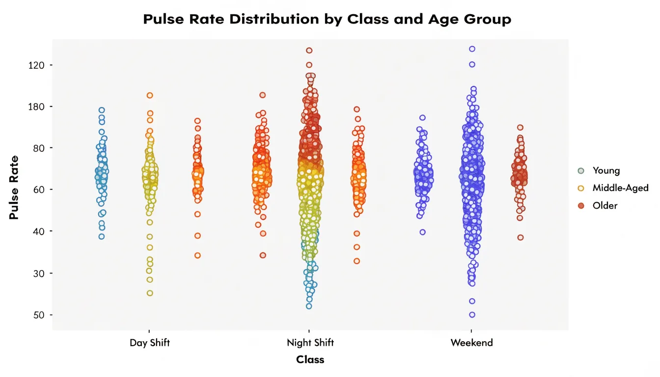
Customization happens through keyword arguments:
hue: color points by a second grouping variable.palette: choose a color scheme.sizeandedgecolor: control marker appearance.dodge: separate hue levels side by side within each category to keep overlapping groups readable.
Matplotlib remains available underneath for finer adjustments: retrieve the current axes with matplotlib.pyplot.gca and modify axis labels, tick rotations, titles, and grid lines directly. You can also layer a swarmplot over a violinplot or boxplot to combine summary statistics with individual observations.
For larger datasets, set a smaller marker size and choose an appropriate figure size through matplotlib.pyplot.subplots so dense categories do not overflow. When saving, use matplotlib.pyplot.savefig with a high DPI value for publication-ready output.
R Beeswarm Plots
The ggbeeswarm package extends ggplot2 to produce beeswarm plots within a grammar-of-graphics workflow. Once installed and loaded with library(ggbeeswarm), the primary function is geom_beeswarm(), which takes the place of geom_point() in a standard ggplot call—for example, ggplot(data, aes(x = category, y = value)) + geom_beeswarm().
Several arguments control the layout:
cex: scales the spacing between points; larger values push points further apart.priority: controls the order in which points are placed, with options such as"ascending","descending","density", and"random", affecting how tightly the swarm packs.method: selects the algorithm that computes the offsets.groupOnX: determines whether swarming is calculated along the x-axis for vertical columns or along y for horizontal groupings.corral: confines points within category boundaries when datasets are large, with options like"none","gutter","wrap", and"width"controlling overflow.
Standard aesthetics (colour, shape, size, alpha) pass directly, and the geom composes with facets, scales, themes, and layers such as stat_summary() for medians. Related geoms include geom_quasirandom() for quasirandom jittering. Saving with ggsave() and styling follow standard ggplot2 conventions.
Avoiding Common Mistakes
Three common pitfalls can distort a beeswarm plot:
- Axis truncation: Starting a continuous axis at a value above a meaningful baseline compresses or exaggerates differences between points. Let quantitative axes begin at a sensible baseline, or, when zooming in is necessary, label the axis clearly and note the truncation.
- Excessive random jitter: Beeswarm layouts already offset points deterministically to prevent overlap. Adding aggressive random jitter on top of that displacement can suggest variation that does not exist or detach a point from its true value. Keep offsets tied to the collision-avoidance algorithm.
- Poor color contrast: Low-contrast palettes make it hard to distinguish groups and can render the plot inaccessible to people with color vision deficiencies. Choose palettes with adequate luminance separation, test them against colorblind simulations, and pair color with shape or direct labeling where possible.
Real World Applications
In customer feedback analysis, teams collect star ratings or satisfaction scores across products, regions, and time periods. Plotting each rating as a dot shows immediately whether a product has a solid block of five-star reviews with a small tail of angry ones, or a broad smear of three-star ambivalence. Segmenting the plot by cohort turns it into a diagnostic tool: support teams can spot the specific rating band where complaints concentrate, and product managers can compare release versions to see whether dissatisfaction is spreading or shrinking.
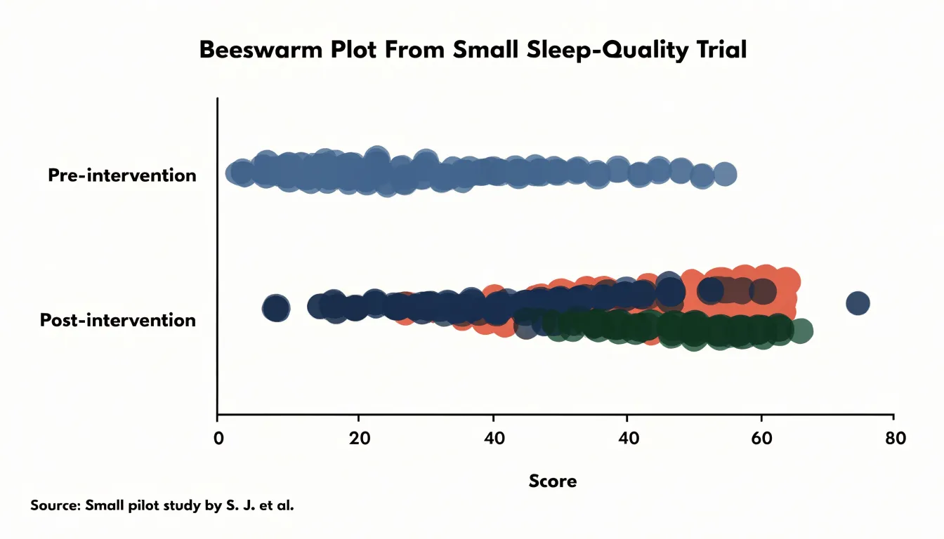
In wellness and clinical research, small sample sizes make every data point valuable. Consider a trial testing essential oil efficacy for sleep quality or anxiety with thirty or forty participants, where a handful of strong responders could pull the mean away from the typical experience. A beeswarm plot of pre- and post-intervention scores places each participant’s outcome on display, showing responders clustered on one side, non-responders on the other, and outliers at the extremes. Splitting the plot by treatment arm or dosage group makes efficacy patterns and individual variability visible in ways that tables of p-values cannot convey, including participants who experienced little or no benefit.
Dashboard Overview
Embedding a beeswarm plot within a business dashboard requires adequate room for points to spread perpendicular to the value axis without crowding and enough span for the variable’s range. Directly above or beside the swarm, a compact summary strip with median, quartiles, and count gives stakeholders an anchor before they examine individual dots.
Interactive and contextual features make the dashboard view actionable:
- Tooltips and brushing: Hover tooltips that reveal each observation’s label and exact value turn the plot into an exploratory instrument, while brushing or filtering by category lets viewers isolate segments in place.
- Companion charts: Linking the swarm to a small histogram or box plot of the same variable supports cross-checking patterns.
- Reference lines and units: Clear axis units and contextual lines marking targets, thresholds, or benchmarks help viewers interpret outliers and clusters against business expectations.
- Consistent controls and guidance: Place filter controls consistently with other dashboard widgets, and include a brief caption noting that swarm width indicates local point concentration to lower the learning curve for non-technical audiences.
Frequently Asked Questions
What is a beeswarm plot and how does it work?
A beeswarm plot places one marker per observation along a value axis and displaces points perpendicular to that axis to prevent overlap. The algorithm sorts points and searches outward for the nearest free position, keeping each point as close to the central axis as geometry allows.
When should I use a beeswarm plot instead of a box plot?
Use a beeswarm plot when sample sizes are moderate, distribution shape matters, and viewers need to see exact observations rather than summary statistics. Box plots remain better for large numbers of groups, very large datasets, or precise quartile comparisons.
What sample size works best for a beeswarm plot?
The practical sweet spot is roughly twenty observations up to several hundred. Below about twenty points, a simple strip or dot plot may convey as much, and above several hundred points the offsets can begin to distort the chart.
How do you handle large datasets in a beeswarm plot?
Establish a threshold—often a few hundred points per category or value bin—beyond which the swarm no longer communicates clearly. Then downsample and document it in the caption, switch to a density or violin plot, or reduce point radius or cap maximum swarm width in borderline cases.
How do I create a beeswarm plot in Python or R?
In Python, Seaborn’s seaborn.swarmplot produces the visualization directly, with options like hue, palette, size, edgecolor, and dodge. In R, the ggbeeswarm package’s geom_beeswarm() works within ggplot2, with arguments such as cex, priority, method, groupOnX, and corral.
What common mistakes should I avoid when making a beeswarm plot?
Avoid axis truncation that compresses or exaggerates differences, excessive random jitter on top of the deterministic offsets, and poor color contrast. Use adequate luminance separation, test palettes against colorblind simulations, and pair color with shape or direct labeling where possible.
Tony Astor
Tony writes about data visualization and the tools people use to build charts and dashboards. More about Data Illustrator