Bar Chart: What It Is and When to Use It
 By Tony Astor ·

Bar Chart
A bar chart is a graphical display that uses rectangular bars to represent data across distinct categories, where each bar’s length is proportional to the value it represents. Bars share a common zero baseline and consistent scale, enabling fast visual comparison of magnitudes across discrete groups such as sales by region or survey responses by category.
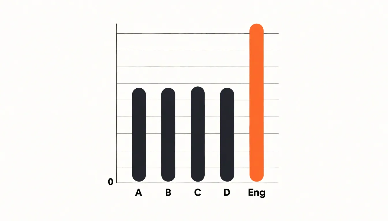
Table of Contents
The Basics of Bar Charts
A bar chart is a graphical display that uses rectangular bars to represent data across distinct categories. Each bar corresponds to a single category, and the length of that bar is proportional to the value it represents. When the bars are oriented vertically, the categories typically run along the horizontal axis, while the values are read against the vertical axis. Horizontal orientation reverses this arrangement, which can be helpful when category labels are long. In either case, the essential relationship stays the same: longer bars signify larger values, shorter bars signify smaller values, and the eye can compare magnitudes immediately without reading individual numbers.
The purpose of the bar chart is comparison across discrete groups. Because the bars share a common baseline and a consistent scale, differences in length translate directly into differences in quantity. This makes the form well suited to data such as sales by region, survey responses by category, or counts of items by type. The discrete nature of the categories matters: each bar stands alone, and there is no implication that the categories blend into one another along a continuum.
Simple design follows from this purpose. A clear bar chart usually includes a labeled axis for the categories, a labeled axis for the values, a consistent starting point at zero for the bars, and enough spacing between bars to keep them visually distinct. Color can highlight a particular category or group, though a single uniform color often serves better when the goal is straightforward comparison. Gridlines and value labels are optional aids that help readers estimate lengths more precisely.
Keeping the design uncluttered supports the chart’s core strength: fast, intuitive visual comparison. When bars are cleanly drawn and scaled consistently, viewers grasp relative magnitudes in a glance, which is exactly the kind of immediate insight a bar chart is meant to deliver.
How Bar Charts Work
A bar chart translates a data table into a spatial comparison by assigning each discrete category to one axis and its corresponding numerical value to the other. When the categories are listed along the horizontal axis, the chart is a column chart; when they run down the vertical axis, the bars extend left to right. Either orientation preserves the essential mechanism: each category becomes a bar whose length or height is proportional to its value against a shared baseline, typically zero. That shared starting point is what makes the comparison fair, because every bar is measured from the same reference and differences in length correspond directly to differences in magnitude.
The value axis carries a regular scale with evenly spaced tick marks, so a bar twice as long as another represents twice the quantity, provided the scale begins at zero. Truncating the axis exaggerates differences and distorts the message, which is why analysts treat a zero baseline as a default rule for bar charts. On the category axis, bars are usually separated by small gaps so viewers read each bar as a distinct entity rather than as a continuous trend.
The format suits rapid cognitive processing because length is one of the easiest quantities for the human visual system to estimate. People compare bars side by side without calculation, reading rank order, relative size, and outliers almost instantly. Grouping, sorting categories by value, or stacking bars adds further structure while keeping the underlying encoding intact. This makes bar charts effective for comparing a handful to a few dozen categories, where the goal is a clear ranking or distribution rather than a continuous pattern over time.
Main Parts of a Bar Chart
Every bar chart is built from a set of interconnected anatomical elements, and understanding these parts is the first step toward reading and creating charts that communicate clearly. The horizontal x-axis typically carries the categorical dimension of the data, such as product names, regions, or time periods, while the vertical y-axis usually represents the quantitative measure, such as sales figures or counts. Together these two axes establish the coordinate space in which the data lives, giving each value a defined position that the eye can locate and compare.
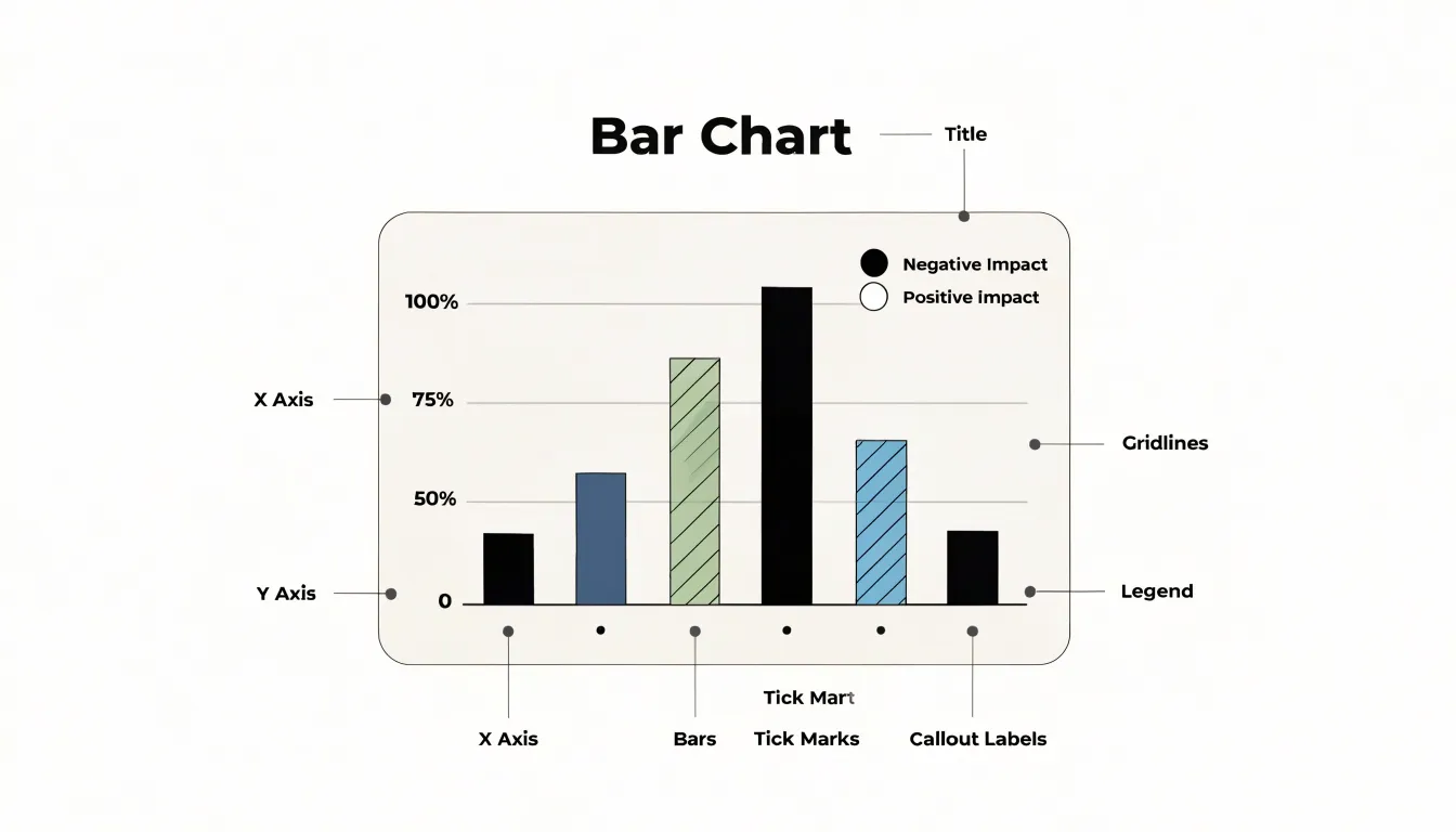
Within that space, the data bars themselves form the visual centerpiece. Each bar’s length or height corresponds to the magnitude of the value it represents, and the bars are drawn against the axis baseline so that comparisons remain fair and intuitive. Tick marks punctuate the axes at regular intervals, anchoring the scale and helping viewers translate a bar’s endpoint into a specific number. Gridlines extend from those tick marks across the plotting area, providing subtle horizontal or vertical guides that make it easier to trace a bar back to its value without straining to estimate.
The descriptive labels complete the picture. Axis titles state what each dimension measures and, where relevant, the unit of measurement, while individual tick labels name the categories or list the numeric intervals. A chart title frames the overall message, and annotations or a legend can clarify individual series when multiple groups appear. Consistent typography, readable font sizes, and clear spacing between labels all contribute to legibility, especially when categories are numerous or names are long. When every one of these elements works in concert, the chart becomes largely self-explanatory, allowing readers to grasp the data’s pattern quickly and accurately without needing additional explanation in the surrounding text.
Vertical Bar Charts
Vertical bar charts, also known as column charts, are particularly effective for displaying standard data sets over time or for small category sets where a natural left-to-right reading order applies. The vertical orientation aligns with the conventional way most audiences read information: from left to right and top to bottom. This makes the chart immediately intuitive, as the eye follows the progression of bars along the horizontal axis, which typically represents time periods or distinct categories. For chronological data, such as monthly sales figures or quarterly revenue, the left-to-right flow mirrors the passage of time, allowing viewers to quickly grasp trends, patterns, and comparisons across periods. Each bar’s height corresponds to the value, and the consistent width and spacing of bars facilitate direct comparison. When the number of categories is small—say, fewer than ten—vertical bars keep the chart uncluttered and ensure that labels remain legible without rotation. The vertical format also accommodates longer category names more gracefully than horizontal bars, as labels can be placed beneath each column and read horizontally without overlapping. Additionally, vertical bars are well-suited for showing part-to-whole relationships when stacked, or for highlighting differences between positive and negative values with bars extending above and below a baseline. The familiarity of the vertical bar chart means it requires little explanation, making it a reliable choice for reports, presentations, and dashboards where clarity and quick comprehension are paramount. By leveraging the natural reading order and the ample space for labels, vertical column charts provide a straightforward and effective way to present standard data sets over time or across small, ordered categories.
Horizontal Bar Charts
When category labels run long, the horizontal orientation of a bar chart becomes a practical necessity. Vertical columns place labels along the x-axis beneath each bar, and once names exceed a few words, those labels must be rotated or truncated to fit side by side. Rotated text forces readers to tilt their heads, while truncation hides information behind ellipses. Flipping the axes moves the labels to the vertical plane on the left, where each name occupies its own row. Text reads naturally from left to right, wrapping or extending into the margin as needed, and the chart keeps a clean horizontal baseline without overlap.
This same flip supports long ranked lists. When a dataset contains dozens of categories arranged by value, vertical columns compress into a crowded strip where bars become thin and gaps disappear. A horizontal layout gives every row a consistent height, so even thirty or forty entries remain legible. The ranking reads top to bottom, matching the way people scan ordered lists, and the bars extend rightward from a shared baseline, making relative lengths easy to compare at a glance.
The horizontal visual plane also distributes space more evenly. Long labels sit in a reserved gutter on the left, while the plotting area on the right stays uncluttered and free of text collisions. Readers can trace a single row from label to bar without crossing other elements. Sorting the rows by value turns the chart into a clear ranking, with the largest or smallest entries anchored at the top where attention lands first. Together, these qualities make the horizontal bar chart the default choice for extended category names and large ordered datasets.
Grouped Bar Charts
Grouped bar charts arrange bars into clusters, with each cluster representing a main category and each bar within the cluster representing a subgroup or secondary variable. This structure lets readers compare values across subgroups within a single category while also scanning trends across categories as a whole. The visual proximity of bars inside a cluster makes within-category comparisons immediate, and the consistent ordering of bars from cluster to cluster supports cross-category reading. A legend or direct labeling should identify each subgroup clearly, and the color palette should keep subgroups distinguishable without competing for attention.
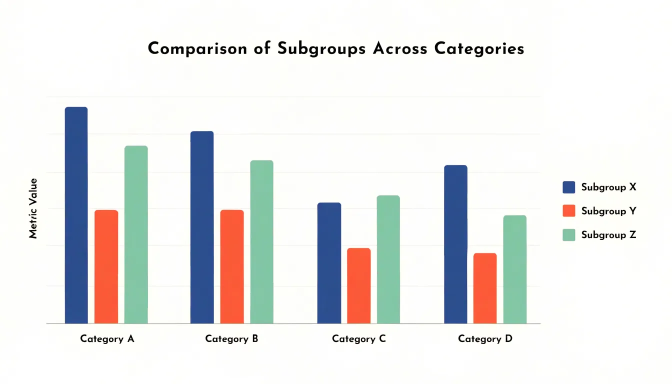
The number of subgroups per cluster has a direct effect on readability. Two to four bars per group usually work well; beyond that, bars grow thin and the chart becomes crowded. When more subgroups are essential, consider facet grids or small multiples instead of forcing everything into a single crowded frame. Consistent bar widths and equal spacing between clusters help the eye separate groups from subgroups. Ordering categories by a meaningful value, such as the largest subgroup total or an overall average, gives the chart a narrative direction rather than an arbitrary sequence.
Design choices should reduce cognitive load. A shared y-axis starting at zero preserves honest comparison, and light gridlines can guide value estimation without dominating the plot. Direct value labels work best when clusters are few; otherwise, a well-scaled axis suffices. Avoid decorative patterns inside bars and limit the palette to a few distinct hues. Sorting subgroups consistently across clusters also aids comparison. When the message concerns a single subgroup, highlighting it in a stronger tone while muting the others can focus attention. Used with restraint, grouped bar charts give readers a compact, orderly way to evaluate several secondary variables across main categories at once.
Stacked Bar Charts
Stacked bar charts arrange sub-bars end to end within a single total bar, so each category reads simultaneously as a sum and as a set of components. The full length of the bar represents the cumulative total for that category, while the internal segments show how much each sub-group contributes to that total. A viewer can compare overall magnitudes across bars by looking at their heights or lengths, then examine the internal composition of any single bar by tracing the colored segments from bottom to top. This dual reading makes stacked bars useful whenever a dataset describes parts that combine into a meaningful whole, such as revenue broken down by product line, survey responses split across answer choices, or monthly output divided among production facilities. Because every segment shares the same baseline direction, the stack communicates accumulation directly: each segment’s top edge marks the running subtotal up to that point, and the final edge marks the grand total. Designers typically order segments consistently across all bars, placing the largest or most stable component at the base so that comparisons between adjacent bars remain easy to follow. The resulting chart packs two layers of information into a compact space. The overall bar length answers questions about totals, while segment lengths answer questions about shares and relative contribution. Readers can spot which category is largest overall and, in the same glance, see whether that dominance comes from one large component or from several moderate ones. This efficiency explains why stacked bars appear so often in reports and dashboards where the goal is to show both the size of each group and the mix of its constituent parts.
Segmented Percent Bar Charts
Segmented percent bar charts normalize total bar heights to 100%, allowing readers to compare percentage distributions across categories rather than absolute quantities. In a standard segmented bar chart, each bar’s height reflects a total count, and its segments show how that total divides among subcategories. When those totals differ widely, however, comparing segment sizes becomes difficult, since a small segment in a large bar can visually outweigh a larger segment in a small bar. Normalizing every bar to the same height removes this distortion and puts the focus squarely on relative proportions. Each bar becomes a self-contained distribution, and segments can be compared directly from one bar to the next.
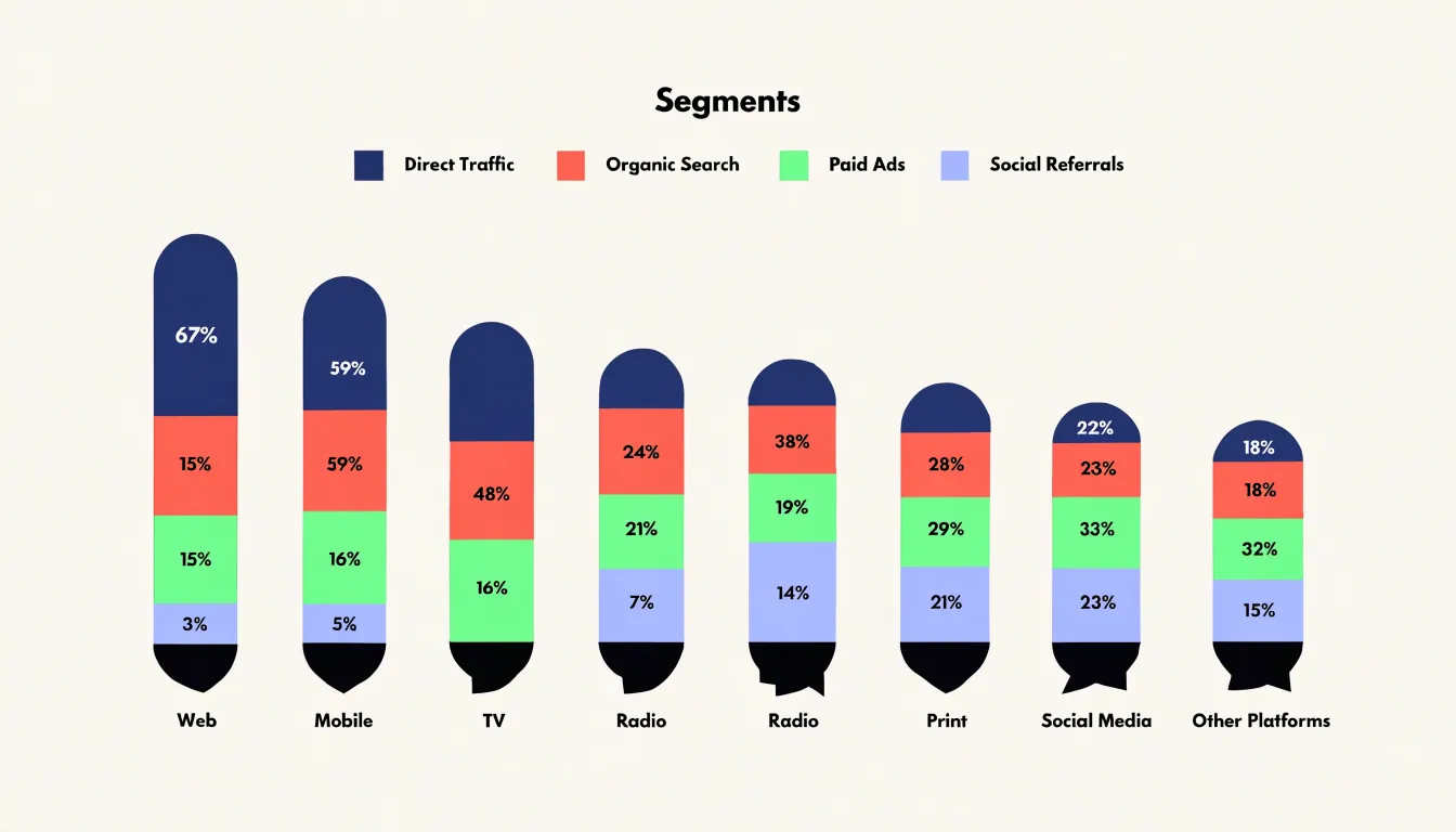
This format is especially useful when the question at hand concerns composition rather than volume. A survey might ask how preferences differ between regions, age groups, or time periods, where the underlying sample sizes vary considerably. By converting each group’s results into percentages of its own total, the chart highlights whether one group leans more heavily toward a particular response, independent of how many respondents each group contains. The same logic applies to market share across product lines, budget allocation across departments, or demographic breakdowns across neighborhoods.
Constructing these charts requires a few practical considerations. Segment order should remain consistent across bars so that readers can track the same category from left to right. Labels or a legend should identify each segment clearly, and the percentages within a bar should sum to 100, with rounding handled carefully so that discrepancies do not confuse viewers. Color choices should keep adjacent segments distinguishable while avoiding visual clutter. When many subcategories exist, grouping small segments into an “other” category often improves readability.
The main strength of the segmented percent bar chart lies in its capacity to make proportional patterns visible at a glance. Readers can scan across bars and immediately see shifts in composition, spotting which groups concentrate on particular categories and which spread their weight more evenly. This makes the chart a compact and effective tool for comparative distribution analysis.
When to Use Bar Charts
Bar charts work best when the data has natural boundaries between categories. Sales figures for five regional offices, survey responses across demographic groups, or the number of support tickets filed by department all share a quality that suits bars: each item exists as a separate, countable unit. When your dataset looks like a list of labeled values rather than a continuous flow, a bar chart turns that list into an immediate visual comparison. The reader can scan lengths side by side and grasp relative size without studying numbers.
Ranking tasks are another strong fit. If the goal is to show which product leads the market, which branch hits its target, or which marketing channel returns the most revenue, a horizontal bar chart arranged from largest to smallest makes the hierarchy obvious at a glance. Sorting the bars transforms raw comparison into an ordered story, and the reader instantly sees the leaders, the middle pack, and the laggards. This ordered presentation is especially useful in reports where decision-makers need to identify top performers quickly.
Bar charts also handle distinct temporal changes well, provided time is split into separate, meaningful periods. Quarterly earnings, monthly website visits, or annual headcount figures each represent a self-contained slice of time, and grouped bars can compare the same period across different years or segments. The discrete bars emphasize that each period is a separate measurement rather than a continuous trend, which supports a factual, period-by-period reading of the data. When the data fits these conditions, a bar chart delivers clarity that few other formats can match.
When to Avoid Bar Charts
Bar charts carry a specific set of assumptions, and those assumptions begin to fail once the data moves away from discrete categories and simple magnitudes. A bar chart assigns each category a single value and encodes it as length, which works well for comparisons like counts per region or revenue per product. Problems arise when the underlying data describes a continuous process rather than a set of distinct groups.
Continuous distribution trends are one clear case. If you are tracking how a variable evolves across a spectrum, such as temperature readings across a day or customer spending across income brackets, a bar chart forces that continuum into arbitrary bins. The resulting bars suggest sharp boundaries between adjacent groups, while the actual underlying change may be smooth and gradual. Line graphs preserve the sense of flow and slope that the data genuinely has.
Highly dense time series present a related difficulty. When a dataset contains hundreds or thousands of timestamped observations, bars become thin slivers that crowd together, and patterns such as cyclical rises, sudden dips, or long-term drift are obscured by the visual noise of individual rectangles. Line graphs, or their smoothed variants, condense that density into a readable trajectory and make anomalies stand out against the surrounding trend.
Multi-dimensional relational data poses a different obstacle. A bar chart can display one measure across one grouping variable, and adding a second or third dimension typically means stacking, clustering, or color-coding, all of which quickly overload the reader. When the analytical question concerns the relationship between two continuous variables, or the clustering of points across several attributes, a scatter plot reveals correlation, spread, and outliers that bars simply cannot express.
Recognizing these limits helps in choosing a chart that matches the structure of the data, ensuring the visual form communicates the actual pattern rather than distorting it.
Quick Design Checklist
A quick design checklist helps turn the principles of good bar chart construction into repeatable habits. The first item on that checklist is to start the y-axis at zero. Bars encode value through their length, so a truncated axis breaks the visual relationship between bar length and the number it represents. A bar that appears twice as long as another should represent twice the value; when the baseline is shifted upward, small differences get magnified into dramatic-looking gaps that mislead the reader. Starting at zero keeps the chart honest and lets viewers compare lengths with confidence.
Maintaining consistent bar spacing is the next guideline. Equal gaps between bars, and equal bar widths within a series, give the chart a steady visual rhythm that lets readers focus on the differences in length rather than on irregular geometry. Uneven spacing can imply groupings or relationships that do not exist in the data. When bars are grouped by category, the gap within a group should be smaller than the gap between groups, and that rule should be applied uniformly across the whole chart.
Color deserves deliberate attention as well. An intentional color scheme uses hue to carry meaning: highlighting a single category, distinguishing series in a grouped chart, or signaling positive and negative values. Decorative rainbows of color add visual noise without adding information. Limiting the palette and reserving strong colors for the data points that matter most keeps the chart readable and directs attention where it belongs.
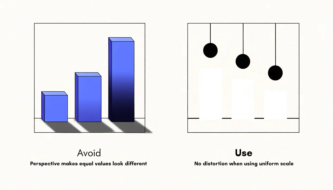
Finally, avoid 3D effects and other forms of visual distortion. Perspective, shadows, and tilted bars change the apparent length of a bar depending on its position in the chart, so two equal values can look different. Flat, two-dimensional bars preserve the direct correspondence between length and value, which is the whole point of the form.
Frequently Asked Questions
What is a bar chart used for?
A bar chart uses rectangular bars to represent data across distinct categories, with bar length proportional to the value it represents. It is designed for comparing discrete groups, such as sales by region or survey responses by category.
Why should a bar chart start at zero?
A zero baseline makes comparison fair because every bar is measured from the same reference, so differences in length correspond directly to differences in magnitude. Truncating the axis exaggerates differences and distorts the chart’s message.
When is a horizontal bar chart better than a vertical one?
Horizontal bar charts are better when category labels are long or when you have a long ranked list, because labels sit on the left and read naturally without rotation or truncation. They also keep many rows legible, with ranking reading top to bottom.
What is the difference between a grouped and a stacked bar chart?
A grouped bar chart clusters bars so you can compare subgroups within each main category, while a stacked bar chart places sub-bars end to end within one total bar. Stacked bars show both the cumulative total and how much each component contributes.
What is a segmented percent bar chart used for?
It normalizes total bar heights to 100% so readers can compare percentage distributions across categories rather than absolute quantities. This is useful when the question concerns composition rather than volume, such as survey preferences across groups with different sample sizes.
When should you avoid using a bar chart?
Avoid bar charts for continuous distribution trends, highly dense time series, and multi-dimensional relational data. In those cases, the bars can force a continuum into arbitrary bins, become too crowded, or overload the reader.
Tony Astor
Tony writes about data visualization and the tools people use to build charts and dashboards. More about Data Illustrator