Bar Chart vs Histogram: Key Differences Explained
 By Tony Astor ·
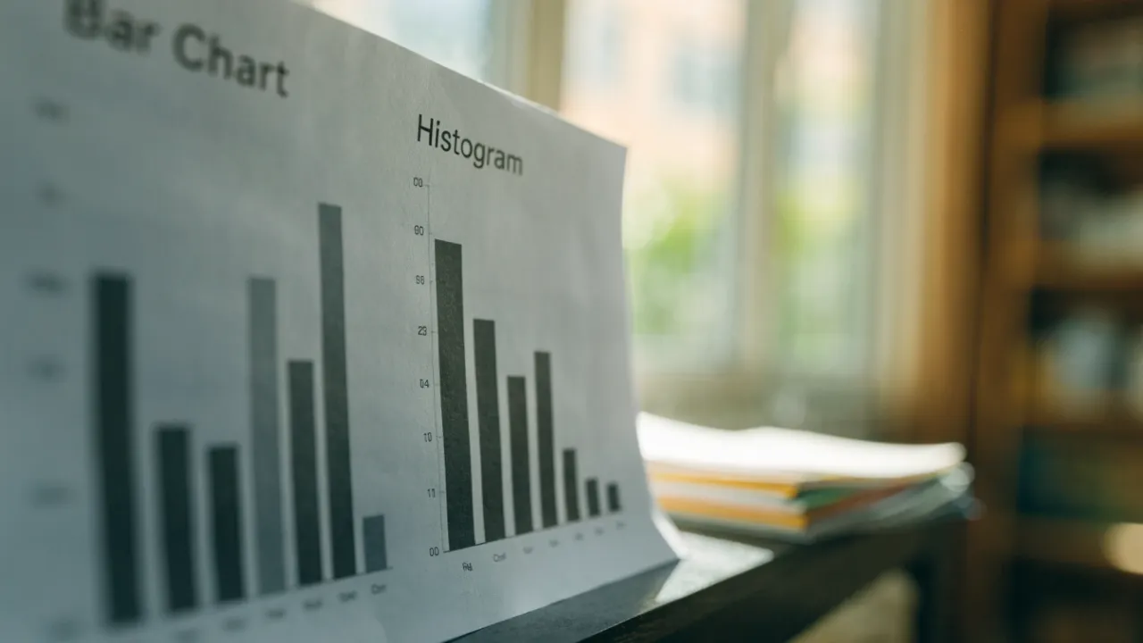
Bar Chart vs Histogram
A bar chart compares discrete categories using separate bars with gaps, while a histogram shows the distribution of continuous numerical data using touching bars called bins. Bar charts use categorical data and allow reordering; histograms use continuous data on a fixed numerical axis, revealing shape, skew, and spread.
Table of Contents
Bar Chart
A bar chart is a graphical tool designed for comparing amounts across distinct categories. It displays discrete variables, meaning variables that fall into separate, non-overlapping groups such as types of fruit, months of the year, or modes of transportation. Each category is represented by a separate bar, and the bars are typically separated by gaps to emphasize that the categories are distinct and not part of a continuous scale.
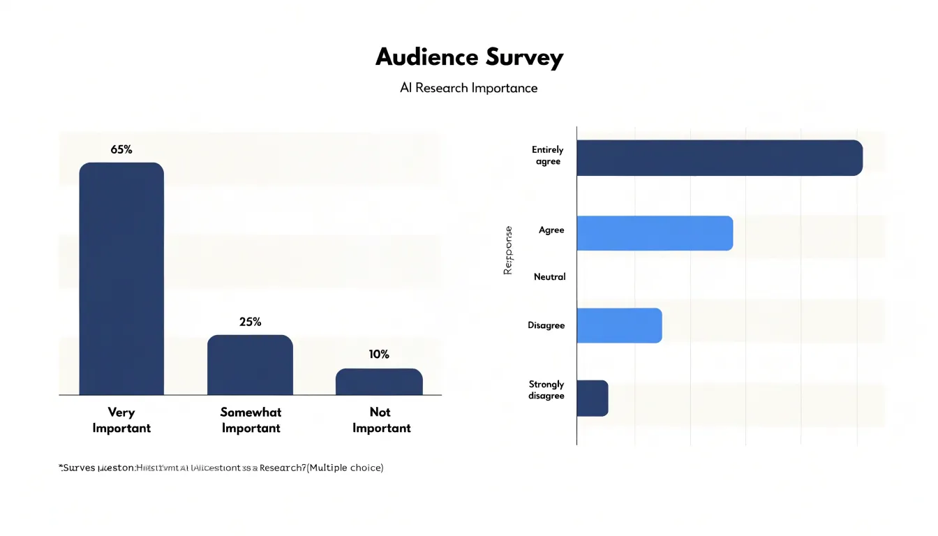
The length or height of each bar corresponds to the value or frequency associated with that category. This visual encoding allows viewers to quickly assess relative magnitudes: a longer bar indicates a larger amount, while a shorter bar indicates a smaller amount. Because the bars are separated, the chart makes it easy to compare individual categories side by side without implying any order or connection between them.
Bar charts can be oriented vertically or horizontally. Vertical bar charts, also called column charts, are common for displaying categories along the x-axis and values along the y-axis. Horizontal bar charts are useful when category labels are long or when there are many categories, as they provide more space for text. In either orientation, the key feature is the separation between bars, which reinforces the discrete nature of the data.
When constructing a bar chart, it is important to start the value axis at zero to avoid exaggerating differences between bars. The bars should be of equal width, and the gaps between them should be consistent. These practices ensure that the visual representation accurately reflects the underlying data and supports fair comparisons.
Bar charts are widely used in business, education, and media to present categorical data clearly. They are particularly effective for showing rankings, identifying the most or least common category, and comparing multiple groups across the same set of categories.
Histogram
A histogram displays how a set of numeric values is distributed across its range. The data is continuous quantitative data, such as heights, temperatures, or response times. To build the chart, the full range of values is divided into a series of adjacent intervals called bins. Each bin covers a span of values, and every observation falls into exactly one bin. The bins sit side by side with no gaps, mirroring the continuous flow of the underlying numbers.
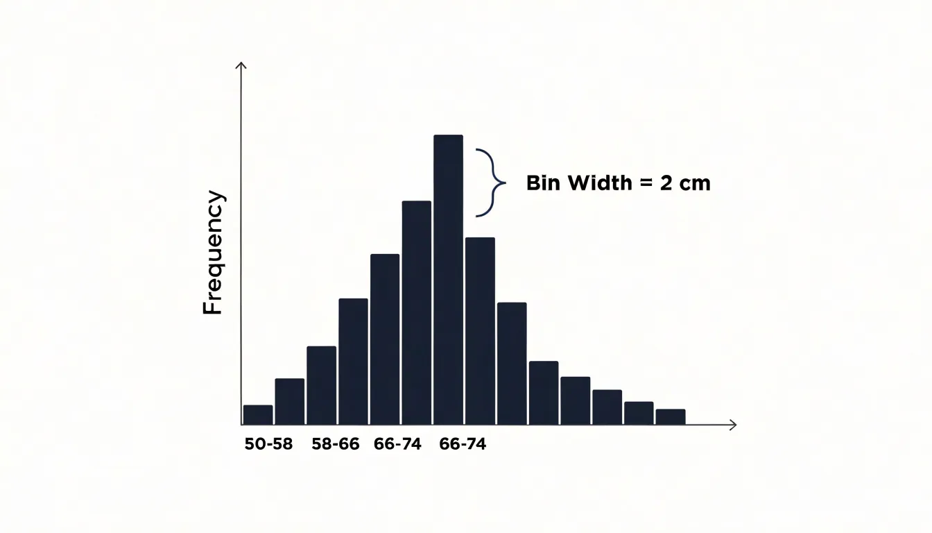
The height of each bar reflects the count or frequency of observations within that bin. When the bars are drawn with widths proportional to the bin ranges, their area also expresses density, which becomes important when bins are unequal in width.
The resulting silhouette reveals the shape of the distribution. A cluster of tall bars on the left with a long tail toward higher values signals skew. A symmetric mound centered on the mean suggests a roughly normal spread. Multiple peaks can point to distinct subgroups inside one dataset. Reading a histogram involves scanning where the mass of the bars sits, how wide the spread extends, and whether any values appear isolated from the main body of data. Because the bins are contiguous, the eye reads the chart as a single continuous shape rather than a set of separate categories. That visual continuity makes the histogram a natural tool for spotting outliers, comparing central tendency across datasets, and judging whether the spread is wide or narrow.
Choosing an appropriate bin width matters, since very narrow bins can look noisy while very wide bins can flatten important detail. With a sensible bin size, the histogram turns a long list of raw numbers into a clear picture of how those values behave across their numeric range.
Categories vs Ranges
The most fundamental difference between a bar chart and a histogram lies in what the horizontal axis represents. In a bar chart, each bar stands for a distinct category, a qualitative label that names a group rather than measuring it. Product types, regions, departments, or brands are typical examples. These categories have no inherent numerical order; you can arrange them alphabetically, by value, or in any sequence you prefer, and the meaning of the chart remains intact.
A histogram’s horizontal axis represents a continuous numeric range divided into bins, such as age brackets of 0 to 9, 10 to 19, and 20 to 29. Every value in the dataset falls within one of these intervals, and the order of the bins is fixed by the underlying numbers along a number line.
This distinction shapes how readers interpret each chart. A bar chart answers questions about which category is largest or smallest, drawing attention to comparisons between discrete groups. A histogram answers questions about how values are distributed across a continuum, revealing patterns such as concentration around a central range, skew toward one end, or multiple peaks. The gap versus no-gap convention reinforces this contrast visually, giving viewers an immediate hint about whether they are looking at separate groups or slices of a continuous whole.
Bar Spacing and Width
In a bar chart, the gaps deliberately placed between bars signal that the categories are separate: apples and oranges sit side by side without blending into one another. The width of each bar is typically uniform, reflecting that each category carries equal standing, while the spacing itself becomes a visual cue that the reader is comparing discrete items rather than tracing a progression along a scale. Bar width in a bar chart is mostly a stylistic decision.
In a histogram, the intervals run directly into one another, so the bars touch, showing that the underlying variable flows continuously from one bin to the next. Here, bin width is a deliberate modeling choice that directly shapes the story the data tells: wider bins group more values together and smooth the shape of the distribution, while narrower bins reveal finer detail but can produce a jagged, noisy profile. Choosing bin size therefore affects how the overall pattern is read, and the touching bars remind the viewer that adjacent intervals are parts of one unbroken scale.
Ordering Data
Because each bar in a bar chart represents an independent group, the sequence in which those bars appear is a design decision rather than a mathematical requirement. An analyst can sort the bars from largest to smallest to highlight the top performers, arrange them alphabetically for quick lookup, or group related categories together to reveal patterns. The chart remains equally valid under any arrangement, since the height of each bar carries the information and the position simply serves as a label. This flexibility makes ordering a powerful storytelling tool: placing the tallest bar first draws the eye immediately, while a deliberate alphabetical order signals a reference chart rather than a ranking.
A histogram operates under a different set of constraints. Its bins occupy specific ranges on a number line, such as age, income, or measurement error, and must run in strict ascending or descending sequence so that the axis reflects the underlying scale. Reordering the bins would break the relationship between position and value, turning a meaningful distribution into a jumble of disconnected intervals. The shape formed by the bar heights—whether a bell curve, a skew, or a bimodal pattern—depends entirely on the bins staying in their natural order. Readers interpret a histogram by scanning left to right along the measured variable, so any rearrangement destroys the visual logic of the chart.
Sorting category bars is a legitimate step in presentation, while sorting histogram bins would misrepresent the data.
When to Use a Bar Chart
A bar chart suits situations where you need to count or compare a manageable number of distinct, non-overlapping items. In practice, this covers a wide range of everyday reporting tasks. A sales manager comparing revenue across four regions, for instance, is dealing with a small set of clearly defined groups. Each region stands alone, the totals can be compared side by side, and the gaps between them are meaningful in themselves. A bar chart lets readers rank regions, spot underperformers, and gauge relative size at a glance.
Survey responses offer another natural fit. When respondents choose among discrete options such as a preferred contact method or a satisfaction rating, the resulting counts belong to separate buckets rather than points along a continuous scale. Plotting those counts as bars makes it easy to see which option dominates, which is rarely chosen, and how large the gaps are between choices.
Bar charts also handle ordered categories well, such as age brackets or education levels, provided the goal is to compare counts within each self-contained group.
When to Use a Histogram
Histograms are the tool of choice for tracking continuous distributions in real-world scenarios. For example, a marketing team analyzing customer age demographics can use a histogram to see whether their customer base skews young, old, or is spread evenly. The shape of the histogram immediately reveals peaks, gaps, and outliers that might be missed in a summary table.
Similarly, educators examining exam score distributions can use a histogram to assess difficulty and identify common score ranges. A bell-shaped curve suggests a typical spread of performance, while a skewed distribution might indicate an unusually hard test or a cluster of high achievers.
In manufacturing or service industries, histograms are invaluable for continuous time-duration measurements, such as the time taken to complete a process or the duration of customer calls. By binning these durations, analysts can spot bottlenecks, measure variability, and set realistic performance targets. Histograms also help in quality control, where they are used to monitor process stability and detect shifts over time.
Axis Labels
Axis labels carry much of the interpretive weight in any chart, and the conventions differ depending on whether the chart displays categories or continuous ranges. On the x-axis, a bar chart displays named categories, whereas a histogram places quantitative bins (such as age ranges or income brackets) whose labels should make the interval boundaries clear to the reader.
The y-axis follows a parallel logic tied to what the chart measures. In both chart types, the vertical axis most often shows total counts or frequencies, answering the question of how many observations fall into each category or bin. When comparisons across groups of different sizes matter, percentages or relative frequencies can replace raw counts, and the axis label should state clearly which measure is in use. Consistent labeling matters here: if one chart in a report shows counts and another shows percentages, each y-axis must say so explicitly, since the visual shapes may look identical while conveying different information.
Clear axis titles complete the picture. The x-axis title should name the variable and, for histograms, note the bin width where relevant. The y-axis title should name the measure, such as Frequency, Count, or Percentage of Respondents. Units, where applicable, belong in the titles rather than scattered among tick labels. Following these guidelines keeps the chart readable and ensures that viewers interpret each axis in the way the data intends.
Example
Start with a small survey dataset covering thirty participants. Each person reports their favorite snack and their age. Imagine the snack column lists categories such as chips, fruit, chocolate, and pretzels, while the age column records values between 18 and 65.
The first visualization groups the snack responses by category and draws a separate bar for each one, with the bar height counting how many people chose that snack. The x-axis holds the snack names, the y-axis holds the counts, and every bar stands alone with a gap between neighbors. This arrangement answers questions about which snacks are popular and how the preferences rank against one another.
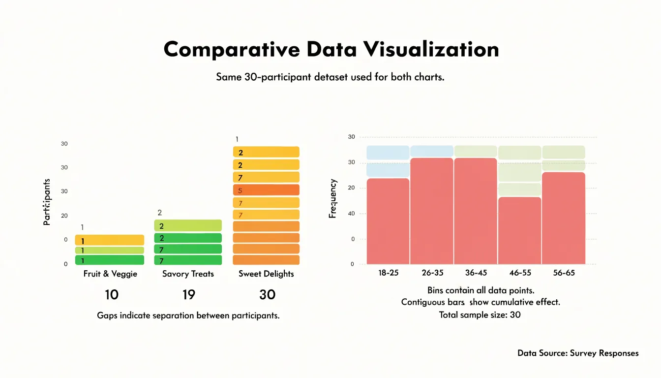
Next, turn to the age variable. Rather than drawing one bar per distinct age, define bins such as 18 to 25, 26 to 35, 36 to 45, 46 to 55, and 56 to 65. Count how many participants fall inside each bin and draw contiguous bars whose widths match the bin ranges and whose heights match the counts. The age axis forms a continuous number line, so the bars touch and together trace the shape of the age distribution. From this histogram, a reader can see whether the sample skews young or old, where the ages cluster, and how spread out the values are.
Placing the two charts side by side makes the distinction concrete. The snack chart treats each flavor as a discrete label with no inherent order, while the age chart treats a numeric variable divided into intervals. The walkthrough also shows practical choices: a bar chart needs a category order that aids comparison, and a histogram needs thoughtful bin widths so the distribution stays readable without hiding detail or adding noise.
Common Mistakes
When people first learn to work with bar charts and histograms, three recurring mistakes tend to appear:
- Leaving gaps between histogram bins: Bar charts separate their bars with small spaces, and that habit carries over easily. In a histogram, however, a gap implies that values could fall between the adjacent intervals, which misrepresents how the underlying continuous data works.
- Reordering histogram bars: Because bar charts often sort categories by size for emphasis, beginners may rearrange histogram bins in the same way. Shuffling bins breaks the connection between a bar’s position along the number line and the range of values it represents, turning a distribution into a misleading arrangement.
- Treating continuous data as discrete categories: Continuous values need to be grouped into intervals that cover the full range without overlap or omission. When someone plots each distinct numerical value as its own separate bar with spaces around it, the result looks like a bar chart and loses the sense of an underlying continuum.
Reading Distribution Shape
The silhouette of a histogram’s bars reveals the distribution’s shape:
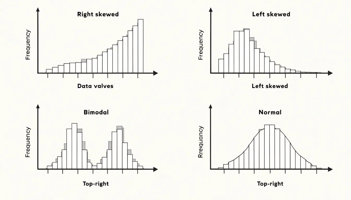
- Right-skewed: When the tallest bars cluster at the left and the heights taper gradually toward the right, a long tail stretches toward higher values. Incomes, housing prices, and waiting times commonly produce this profile, where most observations sit at the low end while a few extreme values pull the tail outward.
- Left-skewed: Bars peak near the right side and the tail trails toward lower values, a pattern familiar from exam scores on a difficult test or ages at retirement.
- Bimodal: Two distinct peaks separated by a valley signal that the dataset likely mixes two underlying groups, such as delivery times from two different warehouses or heights combining men and women. Drawing a histogram makes this split immediately visible, prompting a closer look at how the data was gathered.
- Normal (bell curve): A symmetric mound where bars rise steadily to a central peak, then fall away evenly on both sides. Around 68 percent of values fall within one standard deviation of the mean in this pattern, which underpins much of statistical inference. Spotting symmetry in a histogram is the first step toward deciding whether normal-based methods apply.
Bar charts cannot support this kind of reading because their categories can be rearranged without changing meaning, whereas a histogram’s fixed numeric axis carries genuine diagnostic information about skew, modality, and symmetry.
Choosing Bin Widths
Grouping data correctly is a critical step in constructing a histogram, as bin width directly influences the shape and interpretability of the resulting distribution.
Selecting a bin width that is too wide merges distinct data points into broad categories, which can obscure underlying patterns such as multiple peaks or subtle variations in frequency. For example, in a dataset with two closely spaced modes, wide bins may combine them into a single, misleading peak, suggesting a unimodal distribution when the data are actually bimodal. Wide bins can also smooth over important features like skewness or kurtosis.
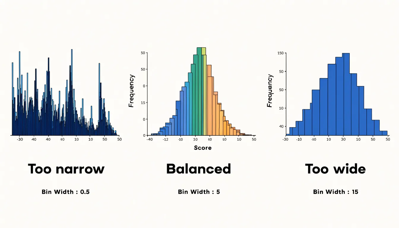
Conversely, a bin width that is too narrow produces a spiky histogram with many empty or low-frequency bins, making it difficult to discern the overall shape of the distribution. This over-granularity can emphasize random noise rather than meaningful trends and exaggerate gaps or outliers, leading to biased visual analysis.
Therefore, the choice of bin width should be guided by the data’s range, the number of observations, and the intended purpose of the visualization. Common rules of thumb, such as Sturges’ formula or the Freedman-Diaconis rule, provide starting points, but analysts should experiment with multiple bin widths to ensure the histogram accurately represents the underlying structure.
Matching Variables
Choosing between a bar chart and a histogram starts with distinguishing qualitative from quantitative data:
- Qualitative data describes categories or attributes and maps naturally to bar charts, where bar height reflects a count, frequency, or proportion.
- Nominal variables, such as eye color, brand names, or vehicle types, have no inherent order.
- Ordinal variables, such as customer satisfaction ratings from poor to excellent or education levels, carry a meaningful sequence but uneven gaps between the ranks.
- Quantitative data represents measurements along a continuous scale, where values can fall anywhere between two points, and requires a histogram.
- Interval variables, such as temperature in degrees Celsius, have equal distances between values but no true zero.
- Ratio variables, such as height, weight, income, or age, have equal intervals and a meaningful zero point.
Collapsing interval or ratio data into isolated categories would discard the distribution’s shape and hide the continuity that defines the measurement. Matching the variable type to the chart type protects the integrity of the data and communicates the structure that actually exists in the numbers.
Quick Comparison
Five dimensions provide a fast reference for distinguishing bar charts from histograms before building or interpreting a visualization:
- Purpose: A bar chart compares discrete categories (such as sales figures across regions or vote counts for candidates), while a histogram shows the distribution of a single continuous variable across a range of intervals.
- Data types: Bar charts use categorical (nominal or ordinal) data; histograms use continuous numerical (interval or ratio) data divided into bins.
- Bar spacing: Bar charts separate bars with gaps to show category independence; histogram bars touch to signal an unbroken continuum.
- Reorderability: Bar chart categories can be sorted (e.g., highest to lowest) without distorting meaning; histogram bins must remain in their natural numerical sequence.
- Visualization goals: Bar charts highlight comparisons and rankings among groups; histograms expose shape, central tendency, and variability within a dataset.
Dashboard Overview
A dashboard overview should begin with a visual clarity checklist that designers apply before any chart reaches a stakeholder. Start by establishing a single, unambiguous focal point for each panel. The viewer’s eye needs a clear entry place, so choose one metric or trend that anchors the chart and let supporting elements recede through lighter weight type and muted fills. Titles should state the takeaway directly, such as “Q3 revenue climbed 12%,” rather than labeling the axis alone, since a takeaway title lets viewers grasp the data story without decoding the chart.
Color carries meaning and demands restraint. Reserve saturated color for the one series or threshold that matters, and render background series in gray so comparisons remain readable without visual noise. Consistent color mapping across every panel on the dashboard prevents viewers from relearning the legend each time they move their eyes. Gridlines, borders, and tick marks belong in a light neutral tone; they support reading values without competing with the data itself.
Labeling deserves similar discipline. Direct labels placed near the data points reduce the back-and-forth between legend and plot, and rounding values to meaningful precision keeps the story legible. Sort categorical bars by value when rank matters, and order time series left to right in alignment with how people read. Every panel should answer one question, so split overloaded charts into focused views rather than layering axes and encodings that force interpretation.
Finally, build in proximity and hierarchy. Group related metrics spatially, size panels in proportion to their importance, and leave generous whitespace so each chart breathes. Test the finished dashboard by asking a colleague to state the main message within five seconds; if they hesitate, simplify the annotations, remove decorative elements, and sharpen the title until the data story reads instantly.
Frequently Asked Questions
What is the main difference between a bar chart and a histogram?
A bar chart compares distinct categories, while a histogram shows how continuous numeric values are distributed across bins. In a bar chart, bars are separated, but in a histogram, bars touch because the intervals form a continuous scale.
When should I use a bar chart instead of a histogram?
Use a bar chart when you need to count or compare a manageable number of distinct, non-overlapping categories, such as revenue across regions or survey response options. Bar charts are effective for showing rankings and comparing categories side by side.
Why do histogram bars touch while bar chart bars have gaps?
Gaps in a bar chart signal that categories are separate, while touching bars in a histogram show that the underlying variable flows continuously from one bin to the next. A gap between histogram bins would imply that values could fall between adjacent intervals, which misrepresents continuous data.
Can you reorder histogram bars to sort them by size?
No. Histogram bins must remain in their natural numerical sequence because reordering them breaks the connection between a bar’s position and the range of values it represents. Bar chart categories, by contrast, can be sorted without changing the chart’s meaning.
How do I choose the right bin width for a histogram?
Bin width should be guided by the data’s range, the number of observations, and the intended purpose of the visualization. Very wide bins can obscure patterns such as multiple peaks, while very narrow bins can look noisy, so analysts should experiment with multiple bin widths.
What can the shape of a histogram tell me?
The shape of a histogram can reveal whether a distribution is right-skewed, left-skewed, bimodal, or roughly normal. It also helps show where values cluster, how wide the spread is, and whether any values appear isolated from the main body of data.
Tony Astor
Tony writes about data visualization and the tools people use to build charts and dashboards. More about Data Illustrator