Area Chart: When to Use It and How to Read It
 By Tony Astor ·

Area Chart
An area chart is a time-series visualization that fills the space between a trendline and a zero baseline, showing both direction and magnitude at once. The line traces movement while the shaded region conveys volume, making it ideal for cumulative totals like monthly revenue, traffic, or usage. Stacked variants layer series to show composition and part-to-whole totals.
Table of Contents
Area Chart
An area chart built around a single series places one continuous trendline across a time axis, with the space between that line and the baseline filled in with color or texture. The line itself carries the story of direction, rising where the metric climbs and falling where it retreats. The shaded region underneath adds a second layer of meaning, giving visual weight to the magnitude of the values at each point in time. A reader can glance at the chart and register both movement and scale in a single impression, which is the central advantage this form offers for time-based reporting.
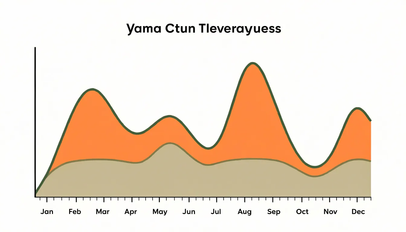
Monthly revenue illustrates the strength of the approach. Each month receives a position along the horizontal axis, and the height of the boundary line shows how much revenue that month produced. The filled area beneath traces the accumulated shape of the year, so a strong quarter appears as a broad, tall mass of color while a slow stretch narrows toward the baseline. Peaks and troughs remain legible as changes in the line’s contour, and the overall bulk of the shaded region conveys the general level of performance without requiring the reader to total individual figures. Seasonal patterns emerge naturally, since recurring high and low months produce a rhythmic profile across the fill.
The single-series restriction keeps the chart focused. With only one trendline and one shaded region, there is no competition for attention and no need for a legend to sort out which color belongs to which category. The eye follows one continuous path from the first period to the last. This makes the form well suited to dashboards and executive summaries, where a quick read of volume and direction matters more than detailed comparison across multiple metrics.
Stacked Area Chart
A stacked area chart builds on the basic area chart by layering multiple data series on top of one another, so that the vertical position of each layer represents the cumulative total of all series up to that point. This stacking approach allows viewers to see two things at once: the overall total across all categories, and how each individual category contributes to that total. Because the layers are stacked, the topmost line of the chart traces the grand total, while the height of each individual band shows the value of that specific series.
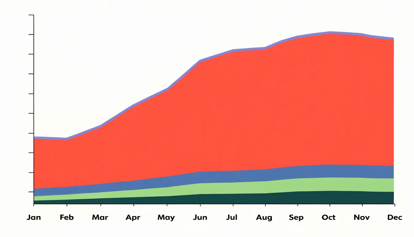
This dual view is especially useful when the goal is to understand how different components add up over a continuous timeline, such as months or years. For example, a stacked area chart could display revenue from multiple product lines, where the total height indicates overall revenue and each colored band shows the contribution of a particular product. The continuous nature of the chart makes it easy to spot periods when one component grows or shrinks relative to others.
However, stacking can sometimes obscure individual trends if the series are not ordered thoughtfully; placing the most stable series at the bottom and the most variable on top often improves readability. Additionally, because the layers are cumulative, comparing the exact values of non-adjacent series can be challenging, so stacked area charts work best when the primary focus is on the total and the relative proportions of components.
100% Stacked Area Chart
A 100% stacked area chart takes the stacked area layout and normalizes every vertical slice so that the categories sum to 100 percent. Each layer represents a category’s share of the whole at that point in time, and the height of any band reflects its proportion rather than its raw value. This normalization makes the chart a tool for tracking composition. When a band widens, that category is gaining share; when it narrows, its share is shrinking, regardless of whether the underlying totals are growing, shrinking, or holding steady.
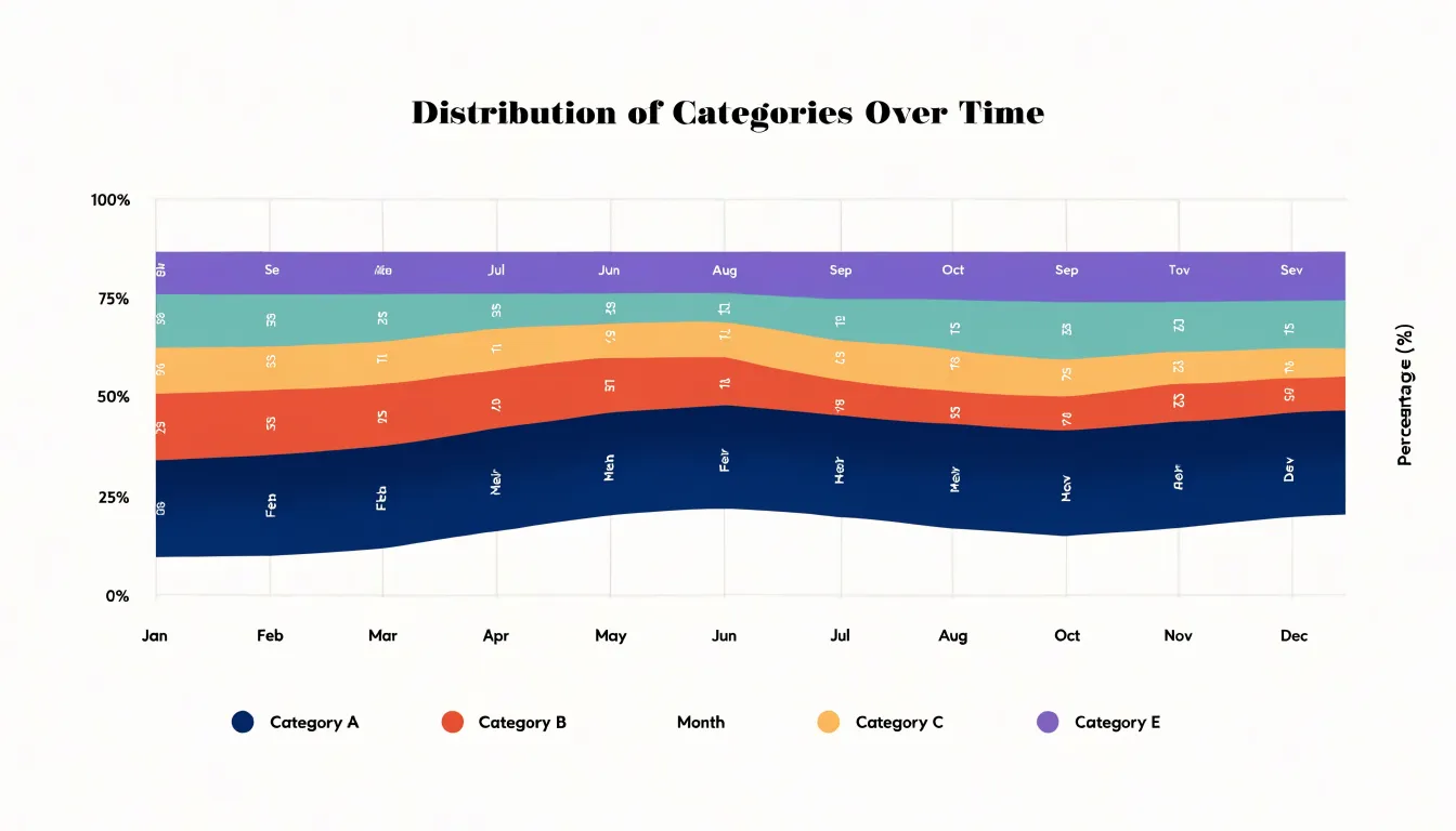
The main advantage appears when absolute magnitudes vary wildly across the timeline. If total volume triples in one period, a conventional stacked area chart shows every band bulging upward, which can obscure the fact that one category’s relative importance may actually be declining. Normalizing to 100 percent removes that distortion. The overall height stays fixed at the top of the plot, so the eye focuses entirely on the boundaries between bands and on how those boundaries migrate up or down over time. Analysts often use this view to answer questions about market share, budget allocation, survey composition, or demographic mix, where the interesting story lives in the proportions rather than in the headline totals.
Reading a 100% stacked area chart benefits from attention to band thickness at specific x positions and to the slope of the dividing lines. A band that holds a steady thickness indicates a stable share, while a slowly tapering band signals gradual erosion of relative position. Because the middle categories are bounded by two moving lines, their shape is influenced by the categories beneath them; as with a standard stacked chart, placing the most stable category at the base usually produces the cleanest visual.
Use this chart when the goal is to communicate relative shares over time and when the total is less important than the mix.
Overlapping Area Chart
An overlapping area chart places two or more series on the same set of axes—each starting from the same baseline rather than stacking—so that their magnitudes can be read against one another across the full width of the x-axis. The central challenge is that a filled area is opaque by nature: where one series sits in front of another, the fill hides whatever lies beneath it. The standard remedy is to reduce the opacity of each fill, often to somewhere between thirty and sixty percent, so that layered regions create a visible blend. Where two translucent fills overlap, the resulting tone signals that both series occupy that region, and a reader can trace either boundary line through the other’s field.
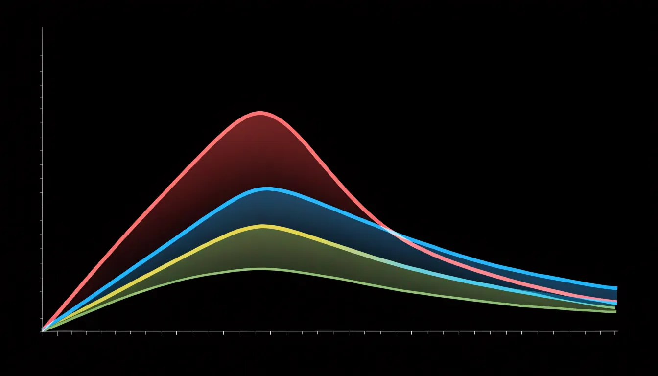
Layering order matters as much as opacity. Series drawn first sit at the bottom of the stack, and their colour will tint every layer above them, so the most important series is often placed on top with a slightly stronger or more saturated stroke. Giving each series a distinct, clearly drawn outline in a darker shade of its fill helps the eye follow individual trajectories even where colours merge. Keeping the palette small, typically three or four series at most, prevents the blended regions from turning into an indistinct muddy wash.
Legends and direct labelling both support interpretation. Placing series names near the right-hand end of each boundary avoids the back-and-forth between legend and plot area. Where a series drops to zero or is temporarily hidden behind a larger one, a subtle pattern such as light hatching can preserve its visibility without adding visual weight. Interactive hover states that raise one series above the others offer a further safeguard on screen.
Streamgraph
A streamgraph is a variation on the stacked area chart in which the layers are displaced around a central horizontal axis rather than resting on a flat baseline. The result reads less like a series of columns and more like a river of data, with each category appearing as a band that swells, narrows, and drifts as values rise and fall over time. Because the shape is organic and continuous, the eye follows the overall flow of the collection while still picking out the movement of individual streams within it. This makes the streamgraph especially suited to storytelling about many categories at once, where the goal is to convey the rhythm of change across a large dataset rather than to read precise values from any single series.
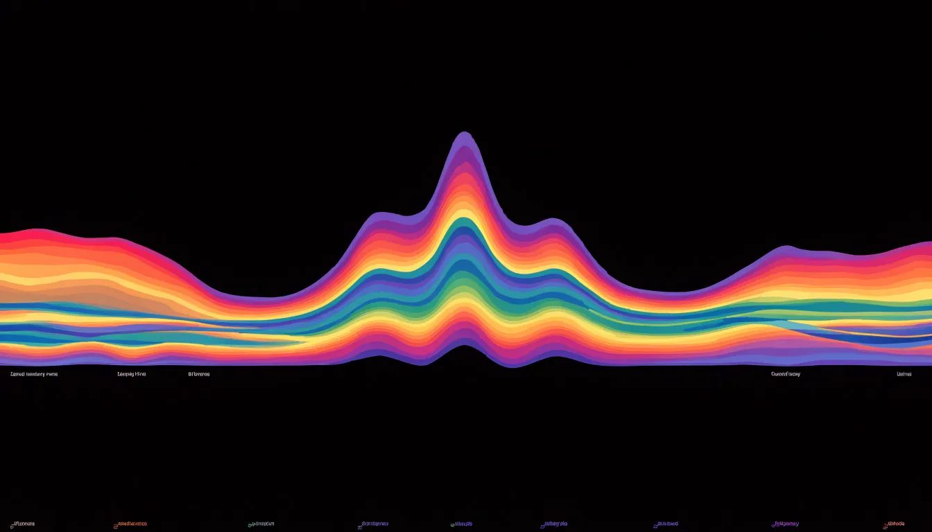
The central axis is the defining design feature. With the bands centered symmetrically, the silhouette above and below the axis forms a balanced shape that draws attention to the relative thickness of each layer. A category that grows pushes its neighbors outward, creating the characteristic undulating profile of peaks and valleys. Smooth interpolation between data points gives the transitions a fluid quality, so that shifts in composition appear gradual and continuous rather than abrupt. Colors distinguish the categories, and the overall silhouette communicates the total volume at each moment.
The technique became widely known through its use in journalism and public data visualization, where it works well for showing the ebb and flow of topics, revenues, populations, or any set of quantities tracked across time. When a dataset contains dozens of categories, the streamgraph’s flowing forms can reveal patterns that a conventional stacked chart would obscure. The trade-off is that exact comparison between layers becomes harder, since the baseline of each band shifts. Designers often pair a streamgraph with interactive highlighting or annotations to help readers trace a particular stream through the overall flow.
Area Chart
An area chart earns its place when the question you are answering concerns magnitude accumulated over time rather than the precise path of a single series. This makes the form well suited to scenarios where cumulative totals matter: monthly revenue, daily website sessions, gallons of water consumed, or hours of machine uptime. In each case the shaded area communicates how much has built up across the period, and the eye naturally compares the size of one block of time against another.
Continuous time-series data is the native territory of the area chart. Because the fill connects successive points into a single continuous shape, the chart implies an unbroken flow from one interval to the next, which matches the way metrics such as traffic, temperature, or inventory actually behave. When observations arrive at regular intervals and the underlying phenomenon never truly stops, the area format reinforces that continuity in a way a scatter of isolated markers cannot.
The chart also handles part-to-whole relationships effectively when several series are stacked. A stacked area chart of energy sources, for instance, shows the growing total demand while revealing how the mix of coal, gas, and renewables shifts underneath it. Use the area chart when the story is about how much, how the total evolves, and how the pieces compose that total across a continuous span of time.
Area Chart
Area charts carry a specific set of limitations that make them a poor fit for certain analytical tasks, and recognizing these situations helps you choose a more suitable visualization. One of the most frequent pitfalls is occlusion. When multiple series are overlaid without sufficient transparency, a lower series can be partially or fully hidden by the series drawn above it. Readers then see only the visible band of the topmost layer while the underlying shapes remain obscured, which distorts the perceived magnitude of each category and makes the chart misleading.
A second difficulty concerns precise data reading. Because an area chart fills the space beneath a line, the eye is drawn toward the overall mass and silhouette rather than to specific values at specific points. Estimating an exact figure along a curved boundary is considerably harder than reading a point on a line, and this problem grows worse when several boundaries crowd together or when the fill colors blend.
For fine-grained comparison between series, line charts offer clear advantages. Lines occupy far less visual space, so multiple series can share a single plot without hiding one another. Each line remains traceable across the entire horizontal axis, and points of convergence, divergence, and crossover stand out plainly. Readers can follow the trajectory of an individual series, judge relative gaps between two series at any given moment, and compare rates of change without the distraction of filled regions.
As soon as the task shifts from cumulative volume toward tracking multiple series closely, spotting small differences, or supporting accurate value estimation, a line chart serves the reader better by keeping the visual field uncluttered and the individual data paths legible.
Area Chart
Reading an area chart accurately begins with understanding what the filled region represents. In a simple, unstacked area chart, the top edge of the shaded area maps directly to a value on the vertical axis, so reading a point means tracing horizontally from that edge to the scale. The baseline sits at zero, and the height of the fill corresponds to the magnitude of the series at any given horizontal position. This direct mapping makes unstacked charts relatively straightforward, provided the axis starts at zero and the scale is consistent along its length. The real interpretive challenges emerge once multiple series are stacked, because each subsequent band no longer rests on a common baseline.
In a stacked area chart, only the bottom series can be read directly against the vertical axis. The band above it represents the difference between two cumulative totals, so its visual thickness, not its vertical position, encodes the value. To gauge an individual slice, you measure the vertical gap between the top and bottom edges of that band at the point of interest, then compare that thickness to the axis scale. A useful habit is to mentally flatten each band to a zero baseline, imagining what its shape would look like if it sat alone on the chart. This helps avoid the common error of reading a band’s upper edge as its value.
Baseline shifts compound the difficulty. When the chart does not start at zero, or when the cumulative stack grows over time, the position of a band’s edges drifts, and the eye tends to conflate vertical position with magnitude. Tracking change over time requires attention to the thickness of a band at successive points rather than its overall trajectory. Comparing the thickness at the start and end of a period reveals growth or decline in that specific series, even when the whole stack rises. Cross-referencing with gridlines, reading across at consistent heights, and checking the axis labeling all reinforce accurate interpretation.
Area Chart
In a multi-series area chart, the colors you select and the opacity you apply determine whether the chart reads as a clear comparison or as a muddled stack of competing shapes. The first step is choosing a palette of distinct hues. Series that sit near one another in the stacking order should have clearly separated hues, so that a reader can tell at a glance where one band ends and the next begins. Palettes built around a consistent saturation and lightness level, varied primarily in hue, tend to work well, since they keep every series visually weighted equally while remaining easy to tell apart. Avoid assigning similar hues to adjacent series, as the boundary between them becomes ambiguous, especially where transparency is involved.
Opacity is the second lever. With transparency applied evenly across overlapping series, overlaps read as blended tones, and the darker regions signal where multiple series coincide. A typical starting point is somewhere in the range of 40 to 70 percent opacity, adjusted based on how many layers are present and how much overlap occurs. When many series stack up, lower opacity values help preserve legibility; with only two or three series, higher values keep colors vivid.
Harmonized hues and consistent transparency let readers trace individual series across the chart and understand the relationship between them.
Area Chart
An area chart encodes value through the size of the filled region between the data line and the baseline, which means that the visual quantity a reader perceives is proportional to the area of the shape rather than to the position of the line alone. For that proportionality to hold, the vertical axis must begin at zero. When the baseline is raised to some value above zero, the height of the filled region no longer represents the full magnitude of the data; it represents only the distance from an arbitrary cutoff. The visual area then shrinks or grows according to that cutoff rather than according to the underlying numbers, and the relationship between the picture and the data breaks down.
The distortion becomes most serious when viewers compare areas across categories or time periods. Suppose one value is twice another, and both sit well above a clipped baseline. Their plotted heights may then appear nearly equal, because most of the true magnitude has been removed from the bottom of the chart. A small change in a large number can look like a dramatic surge, while a large change in a small number can look trivial. Readers who rely on the sweeping visual impression of the fill will form judgments about relative size that the data do not support. Because human perception is highly sensitive to area and volume, these misreadings arise quickly and often go unnoticed, especially when the axis labels are small or absent.
A zero baseline keeps the geometry honest: doubling the value doubles the visible area, halving it halves the visible area. Any chart that uses filled area to convey magnitude should therefore anchor the axis at zero, or clearly mark a break in the axis and signal that the areas are not proportional to the data. Without that safeguard, the chart’s most persuasive feature, its impression of mass, becomes its most misleading one.
Area Chart vs. Line Chart
Area charts and line charts both plot data against a continuous horizontal axis, and both connect successive data points with a line. The visual difference lies beneath that line: an area chart fills the space between the line and the baseline, while a line chart leaves that space empty. This fill changes how the eye reads the graphic. A line invites the viewer to follow the trajectory from point to point, comparing positions on the vertical axis. A filled area creates a visual mass that draws attention to magnitude and volume. When the question is how a total accumulates over a period, the area chart answers it more directly. When the question is exactly where a value sat at a given moment, or how two series cross and diverge at fine scale, the line chart preserves that precision.
The choice also depends on how many series appear in the same frame. A single or stacked area chart reads cleanly when showing volume and composition, whereas line charts handle multiple overlapping series more gracefully without the muddy blends of translucent fills. Precision of tracking favors lines; perception of weight and proportion favors areas.
Practical details reinforce the distinction. Because area charts require a zero baseline to avoid exaggerating apparent volume, they cannot easily zoom in on a narrow value range. Line charts tolerate a narrowed, non-zero axis more readily because readers focus on the path and relative position of the stroke rather than a filled mass. Choosing between them comes down to the story the data should tell: one of accumulation and scale, or one of movement and exact position.
Area Chart vs. Bar Chart
When deciding between an area chart and a bar chart, the key distinction lies in the nature of the data along the horizontal axis. Area charts are designed for continuous data, particularly time series, where the x-axis represents a continuous progression such as dates, months, or years, and the connecting line implies an uninterrupted flow. In contrast, bar charts are suited for discrete categories, where the x-axis consists of distinct, separate groups such as product types, regions, or survey responses. Each bar stands alone, representing a specific category’s value without implying any connection or continuity between categories. The visual separation of bars reinforces the independence of each category.
Structurally, area charts use a continuous filled region to convey total quantity or stacked composition, while bar charts use individual bars whose lengths or heights encode values. This structural difference affects how viewers interpret the data: area charts encourage reading along the continuum, while bar charts invite comparison across discrete items. Moreover, while area charts stack or overlay series to show part-to-whole relationships over time, bar charts can be grouped side by side or stacked to compare discrete categories. Choosing the right chart depends on whether the underlying variable is continuous or categorical.
Area Chart
Area charts earn their place in business reporting because they show both volume and composition at the same time, and a few concrete examples make the pattern clear. Consider website traffic sources tracked month over month. An analytics team plots organic search, paid search, social, referral, and direct traffic as stacked bands. The total height of the stack shows overall traffic volume, while the thickness of each band reveals how much of that traffic comes from each source. When a paid campaign launches and the paid band swells while organic holds steady, stakeholders see at a glance where growth originates. If organic gradually shrinks while social expands, the chart surfaces a shift worth investigating before it becomes a problem.
Sales channel performance follows a similar logic. A retailer might plot revenue by channel such as in-store, e-commerce, marketplace, and wholesale across twelve months. The stacked area reveals seasonal peaks in total revenue and shows which channels drive those peaks. A holiday spike concentrated in e-commerce tells the operations team where to focus inventory and staffing, while a steady decline in one band prompts a review of that channel’s strategy.
Subscription tier growth over quarters is a third strong use case. A SaaS company charts the number of active accounts in basic, pro, and enterprise tiers for each quarter. The rising total reflects overall customer growth, and the relative width of each band shows how the customer base is distributed across tiers. If the enterprise band widens faster than the others, leadership can infer that upmarket motion is working. Shrinking bands at the lower tiers might indicate churn or upgrades, each calling for a different response.
Area Chart
Because an area chart communicates magnitude and composition through large filled shapes, the surrounding canvas needs to stay calm. Reducing gridline noise is the fastest win. Thin horizontal rules in a light neutral tone, drawn only at meaningful intervals, keep the reader oriented without competing with the data. Remove vertical gridlines entirely when categories are labeled beneath the axis, and consider dropping the chart border, which usually adds nothing but visual clutter. If precise reading matters, a few subtle horizontal reference lines serve better than a dense mesh of rules.
Direct labeling eliminates the wasted effort of looking from the legend to the chart and back again. Place category names inside or immediately beside their bands, using a text color with sufficient contrast against the fill. For small bands, a leader line or a callout just outside the plotting area keeps the label legible. Once labels live on the chart, the legend can often be removed, freeing space and removing a redundant decoding step.
Sorting stacks by overall magnitude, with the largest band at the bottom or top depending on your emphasis, produces a stable reading pattern and makes comparisons across charts easier. Logical grouping, such as ranking regions by total volume rather than alphabetically, aligns the visual hierarchy with the story in the data. When categories change order between related charts, keep the sequence consistent so readers can track a band across views.
Together, these refinements reduce visual noise, shorten the path from label to data, and give the stack a predictable structure that supports quick scanning.
Frequently Asked Questions
What is an area chart best used for?
An area chart is well suited to continuous time-series data and to showing magnitude accumulated over time, such as monthly revenue or daily website sessions. The filled area under the line helps communicate both movement and scale in a single impression.
How do you read a stacked area chart?
In a stacked area chart, only the bottom series can be read directly against the vertical axis; for a band above it, the value is encoded by the vertical gap between its top and bottom edges. A useful habit is to mentally flatten each band to a zero baseline and compare its thickness at successive points.
What is a 100% stacked area chart used for?
A 100% stacked area chart normalizes every vertical slice so the categories sum to 100 percent, and each band shows a category’s share of the whole rather than its raw value. Use it when the goal is to communicate relative shares over time and when the total is less important than the mix.
Why should an area chart start at zero?
An area chart encodes value through the size of the filled region, so a zero baseline keeps the visible area proportional to the data. If the baseline is raised above zero, the chart should clearly mark a break and signal that the areas are not proportional to the data.
What is the difference between an area chart and a line chart?
Both plot data against a continuous horizontal axis and connect successive points with a line, but an area chart fills the space between the line and the baseline while a line chart leaves that space empty. Area charts emphasize magnitude and volume, while line charts better preserve precision for tracking exact values and multiple overlapping series.
How can I make an overlapping area chart easier to read?
Reduce the opacity of each fill, often to somewhere between thirty and sixty percent, and give each series a distinct, clearly drawn outline in a darker shade of its fill. Keeping the palette small, typically three or four series at most, helps prevent blended regions from becoming an indistinct muddy wash.
Tony Astor
Tony writes about data visualization and the tools people use to build charts and dashboards. More about Data Illustrator