Alluvial Diagram: Tracking Changes Across Categories
 By Tony Astor ·

Alluvial Diagram
An alluvial diagram visualizes flows of quantities through sequential categories, where the vertical height of each node and connecting band is proportional to the volume it carries. Nodes represent categorical stages along a horizontal axis, and ribbons trace transitions between categories, revealing splits, merges, and pathways across stages.
Table of Contents
Alluvial Diagram
An alluvial diagram presents a flow of quantities through a sequence of categories. Reading one begins with understanding what the height of each element represents. The vertical size of a stream—whether at a node or along a connecting band—is proportional to the volume or count it carries. A thick band means many items, people, or units moving together, while a thin band indicates a smaller share. Because this proportional height is the primary visual cue, scanning the diagram from the widest bands to the narrowest reveals where the bulk of the flow concentrates and where it thins out.
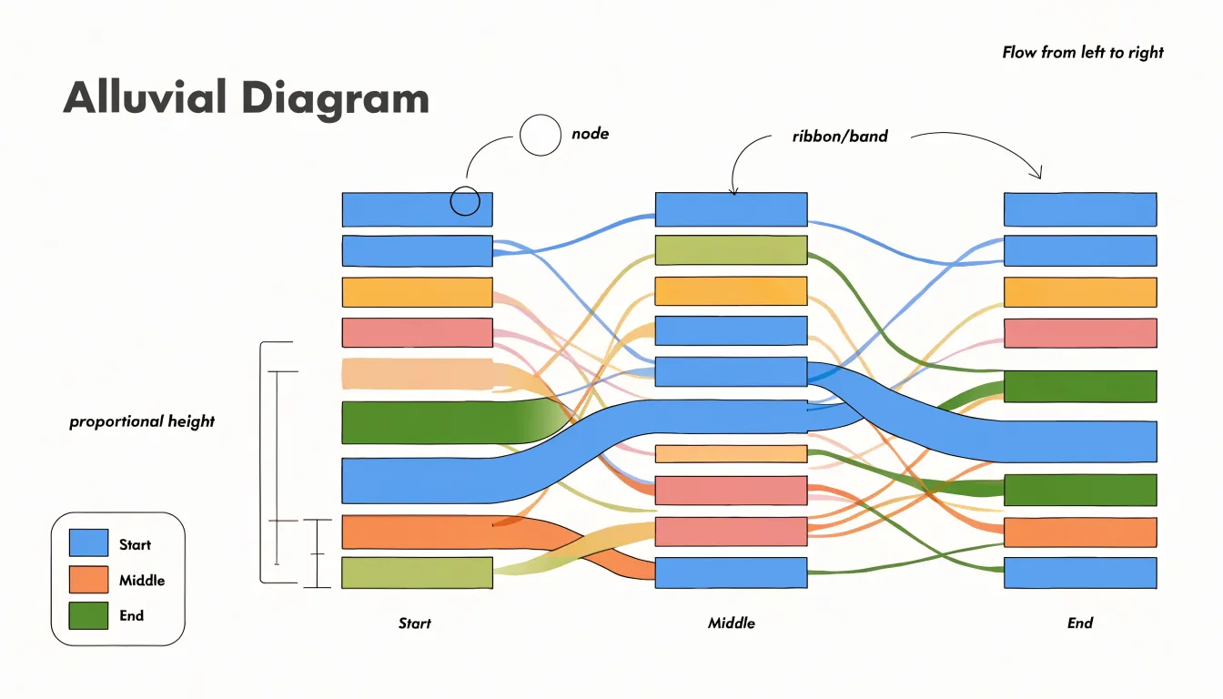
Nodes function as categorical stages along the horizontal axis, dividing the diagram into successive columns that represent time periods, process steps, or classification schemes. Each node groups a set of streams belonging to a single category, and its overall height reflects the total volume passing through that category at that stage. By comparing node heights across columns, a reader can see how totals shift, grow, or shrink as the flow progresses.
Connecting bands (or ribbons) illustrate transitions between groups, tracing a path from a category in one node to a category in the next. Where a band splits, the flow divides among multiple destinations; where bands merge, flows converge into a single category. Following a band across several columns reveals a pathway through the system, and the changing width along that pathway shows gains, losses, or stability at each transition.
Reading the diagram effectively means tracing dominant bands to identify the main routes, noting where splits and merges occur to understand branching behavior, and comparing band widths to judge relative magnitudes at each stage.
Alluvial vs Sankey
Alluvial and Sankey diagrams both visualize flows using proportional widths, yet they serve distinct purposes. Alluvial diagrams focus on categorical changes over time or across discrete stages, such as occupational shifts over decades or party affiliation across elections. The emphasis is on the structure of change: which categories gain or lose members, and how trajectories unfold.
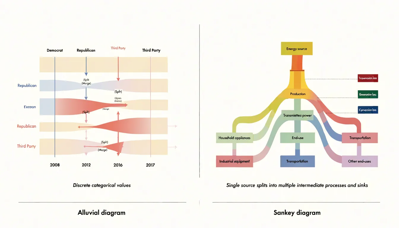
Sankey diagrams, in contrast, emphasize energy or material transfer through a network. Common applications include energy balance studies—where flows of coal, gas, and electricity are tracked from source to end use—or supply chain analyses showing material inputs and outputs. The focus is on the magnitude and direction of transfers, often with a single main flow that branches into smaller ones. Sankey diagrams typically represent a unidirectional process, such as conversion or distribution, and highlight losses or efficiencies at each stage.
These differences shape the visual design:
- Alluvial diagrams use multiple vertical axes to represent discrete time points or classification stages, with flows that split and merge as entities change categories. The layout stresses the categories themselves and their evolution.
- Sankey diagrams usually feature a freer left-to-right progression from source to sink, with nodes representing processes or locations rather than aligned categorical axes.
While alluvial diagrams prioritize categorical transitions and their sequence, Sankey diagrams prioritize quantitative transfer through a system.
Customer Journey Mapping
Customer journey mapping with alluvial diagrams shows how buyers move between preferences, brand loyalties, and sales stages over time. Here, the vertical nodes represent distinct states such as product categories, brands, or funnel stages, while the connecting ribbons represent the cohorts of customers transitioning between them.
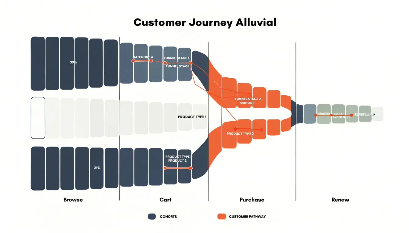
Businesses use these diagrams to trace preference switches across multiple touchpoints. For example, a retailer might map how customers move from browsing to cart to purchase, or how they switch between product lines after a promotion. Analyzing these flows reveals which transitions are most common and which are surprisingly rare.
Another application is visualizing brand loyalty and funnel progression:
- Brand switching: A telecom company might map how customers move between its brand and competitors over several quarters, revealing the impact of pricing changes or service issues.
- Sales funnels: A SaaS provider can track how users progress from trial to paid subscription to renewal, pinpointing where they drop off to enable targeted interventions.
Examining flow thickness helps quantify the impact of marketing campaigns or product changes. A sudden widening of a flow from one preference to another might indicate a successful upsell strategy, while a narrowing flow could signal a bottleneck in the sales process. Over time, repeated diagrams can show broader trends, such as increasing brand switching or the stabilization of customer segments.
Health Trend Tracking
In clinical research, alluvial diagrams track how patient conditions evolve across treatment stages, providing a view of disease progression and therapeutic impact. By recording outcome measures and condition severity at multiple time points—such as baseline, during intervention, and follow-up—researchers can map patient trajectories across severity levels (e.g., mild, moderate, severe).
In chronic disease management, tracking changes in biomarkers, symptom scores, or functional status allows researchers to identify critical transition points. The diagram makes it easy to see the proportion of patients improving, worsening, or remaining stable, while highlighting subgroups that respond differently.
Aggregating data across large cohorts can also uncover treatment-related patterns that summary statistics might miss, such as delayed responses or rebound effects. These insights support evidence-based adjustments to treatment protocols and personalized care plans.
Product Popularity Tracking
Product popularity tracking concentrates on the movement of customers between buying tiers over time. When a shopper who once purchased only entry-level items begins selecting mid-range or premium products, that transition reflects changes in satisfaction, aspiration, and perceived brand value. Rendering each tier as a node across successive periods shows how many customers remain in their original tier, how many ascend, and how many drop away.
Seasonal shifts appear as periodic thickening and thinning of particular flows. A product line that attracts a burst of first-time buyers during a holiday period will show a wide band entering the lowest tier, and subsequent columns reveal whether those buyers stay or dissipate. Over longer horizons, sustained growth in a premium tier signals upward drift in customer confidence, while persistent migration toward lower tiers may indicate price sensitivity or competitive pressure. Comparing flows across several product lines at once lets planners see whether a pattern is confined to one category or reflects broader market behavior.
The practical value lies in forecasting and resource allocation. If the diagram shows steady upward movement within a category, inventory and marketing resources can be shifted toward the higher tiers customers are approaching. If a downward flow dominates, retention efforts can target the segments where defection is concentrated.
Environmental Data Tracking
In ecological and environmental research, alluvial diagrams track how physical areas or biological populations shift across classifications over time.
When applied to land-use classification, the vertical axes correspond to survey years or policy periods, with categories such as forest, cropland, wetland, and urban settlement arrayed along each axis. The ribbons trace how much land passes from one class to another, making visible the gradual conversion of agricultural parcels into developed areas or the recovery of abandoned fields into secondary forest.
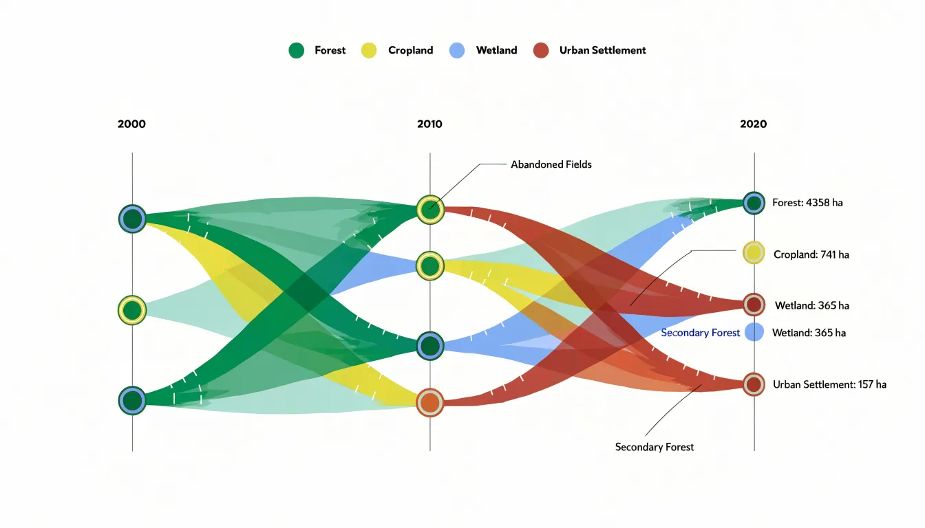
The same structure supports the study of species population migrations across climate phases. Here, the categories along each axis represent habitat zones, seasonal ranges, or thermal bands, and the connecting ribbons show how many individuals or populations shift zones as conditions change. A warming period might produce wider flows from cooler to warmer regions, while a cooling phase reverses that pattern.
Because the diagram preserves both the totals at each stage and the exact pathways between them, researchers can interpret underlying drivers—whether climate change, shifts in land management, or disturbances such as fire and flooding—and communicate these transformations as measurable flows to policymakers and the public.
Data Preparation
Alluvial diagrams begin with categorical data that usually arrives in a wide format: one row per entity, one column per dimension or time point, and values spread across columns to represent category membership at each stage. Before flows can be drawn, this structure must be reorganized into a tidy, long-format table (or aggregated into frequency counts of unique paths). In a tidy long format, each row records a single observation for a single entity at a single stage, with dedicated columns for the entity identifier, the stage, and the assigned category. Most plotting libraries require this structure or a pre-aggregated source-to-target link table.
The categorical dimensions require standardization:
- Consistent vocabulary: Where the same category appears at multiple stages, standardizing its label ensures the flows connect to a shared node name.
- Deliberate ordering: Ordering categories at each stage—alphabetically, by frequency, or by logical sequence—controls how the diagram reads from top to bottom and reduces ribbon crossings.
- Missing values: An entity absent at a given stage may represent a genuine dropout, an unrecorded value, or an out-of-scope category. Analysts must decide whether to drop incomplete rows, insert an explicit “Unknown” or “Dropped” category, or carry previous values forward, as each choice changes which flows appear in the final chart.
Color Choices
Color allows readers to trace continuous pathways across an alluvial diagram. A categorical palette assigns a distinct hue to each major starting node, ending node, or stage category so that streams sharing a common origin or identity carry the same visual signature across the chart. Once a reader learns that a blue stream belongs to a particular group, every subsequent ribbon in that color reinforces the connection without requiring a legend lookup.
Fill opacity is equally important. Solid, saturated fills work well when ribbon counts are low, but in dense diagrams where dozens of streams cross, opaque colors overwhelm the viewer. Semi-transparent fills soften the visual weight of each ribbon and keep overlaps legible. Where streams cross, blended tones reveal the intersection without hiding either pathway, and background grids or node labels remain readable.
To prevent visual fatigue, use muted, evenly spaced palettes so no single stream dominates unintentionally. Limit the palette to a manageable number of hues, grouping minor categories into neutral grays so primary pathways stand out.
Reducing Clutter
When a dataset contains a long tail of low-volume categories, dozens of tiny streams compete for attention, obscuring dominant pathways and creating label overlap. A practical remedy is to aggregate minor categories into a single “Other” bucket.
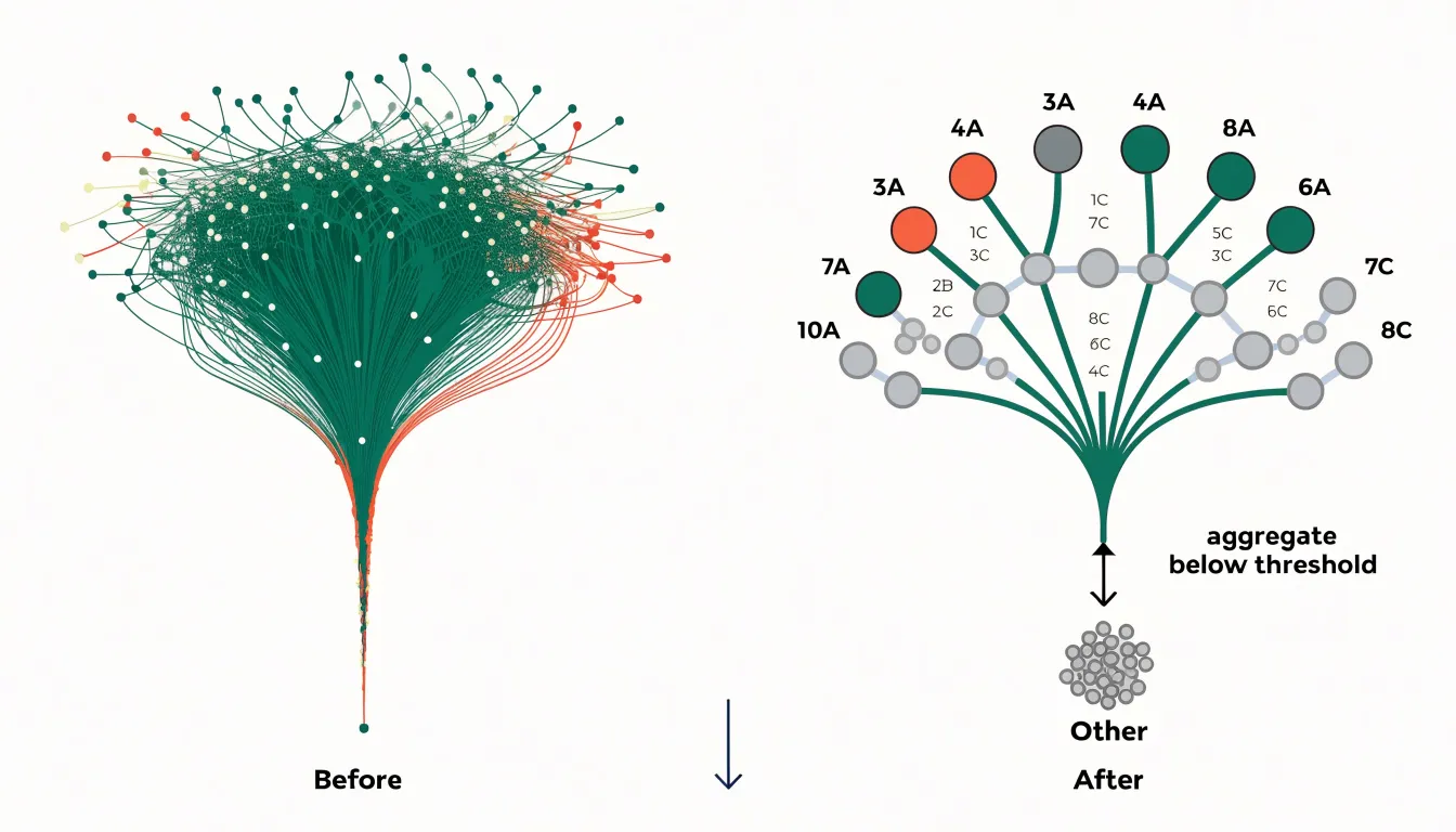
To do this, sort categories by volume or share of total flow, then set a threshold below which categories are merged. Everything beneath that cutoff is channeled into one combined node and ribbon, typically placed at the bottom edge of the vertical axis so it reads as a residual group. This consolidation reduces crossing ribbons, stabilizes node heights, and leaves room to label the remaining major nodes clearly.
The threshold depends on the chart’s context: exploratory analysis warrants a lower cutoff to preserve detail, while presentations and dashboards benefit from a stricter cutoff to keep the focus on major trends. Always document which categories were absorbed into “Other” and their combined magnitude. In interactive tools, allowing users to click and expand the “Other” node on demand preserves both top-level clarity and granular access.
Layout and Sorting
Because every stream connects a node on the left to a node on the right, the vertical position of nodes within each column determines how many streams cross one another. Haphazard ordering produces a web of intersecting bands that obscures individual paths. Careful sorting places related nodes in adjacent positions so their connecting streams run in parallel.
Common ordering strategies include:
- Sorting by magnitude: Ordering nodes by total inflow or outflow pushes the largest categories to the top or center, establishing a clear reading hierarchy while smaller categories settle toward the edges.
- Preserving adjacency: Keeping a recurring category at roughly the same vertical position across consecutive columns lets readers track a stable group straight across the diagram.
- Automated heuristics: Graph-drawing algorithms, such as barycenter or median ordering, iteratively adjust node positions across columns to minimize the total number of stream crossings.
Interactive Features
In web-based dashboards and exploratory tools, interactivity helps viewers navigate dense alluvial diagrams containing dozens of intersecting streams:
- Tooltips: Hovering over a node or ribbon reveals exact counts, percentages, category labels, and supplementary metadata without cluttering the static view with text.
- Hover highlighting: Moving the cursor over a node or ribbon dims unrelated streams and highlights either the single link or the entire multi-stage pathway, letting the eye trace one trajectory across all columns.
- Dynamic filtering: Users can select specific categories, volume thresholds, or source-target pairs to redraw the diagram with only the matching flows, clearing away visual noise.
In browser-based libraries (such as D3.js), implementing these behaviors involves attaching event listeners to SVG elements, maintaining a shared state for the active selection, and using animated transitions during redraws so viewers keep their mental map of the layout as streams enter or exit.
Common Mistakes
Several design errors can make an alluvial diagram difficult to read:
- Inconsistent node spacing: When vertical gaps between nodes vary arbitrarily from one column to the next, readers cannot rely on vertical position to track a category across stages. Uniform spacing and consistent alignment give the viewer a stable frame of reference.
- Poor contrast: If adjacent flows share similar colors, or if node fills sit too close in tone to the connecting ribbons, boundaries blur into an indistinct wash of color. Distinct node borders or strong color differentiation between neighboring flows keeps paths separate.
- Overly complex stages: Including too many sequential steps, or stages with dozens of ungrouped categories, multiplies ribbon crossings into an unreadable tangle. Reduce the number of displayed stages, group minor categories into an “Other” band, or split a dense multi-year diagram into smaller, focused charts.
Presenting Flow Charts
Walking an audience through a complex flow diagram during a live presentation requires deliberate pacing:
- Frame the system first: Before examining specific flows, state what the overall chart represents, what the columns mean, and what units the band widths measure.
- Move in a consistent direction: Guide the audience from left to right along the sequence of stages. Pause at major junctions to name the transition occurring there, using clear spatial language (e.g., “branching into two paths” or “merging into the premium tier”) while guiding their eyes with a pointer.
- Reveal complexity gradually: Build the chart in stages through slide animations, or dim sections not yet under discussion. When a busy cluster of nodes appears, highlight the two or three paths that carry the main takeaway rather than explaining every minor strand.
- Pause for questions at junctions: Check for understanding at complex splits or merges before moving to the next column, as confused listeners tend to disengage early.
- Zoom out to close: Return to the full, un-dimmed diagram at the end and restate the primary conclusion in a single sentence.
Overview and Dashboard
In executive dashboards, alluvial diagrams answer high-level questions about organizational movement—such as customers shifting between tiers, products moving across performance bands, budgets reallocating across departments, or employees changing roles across quarters—patterns that standard KPI tiles and summary tables often hide.
When integrating an alluvial diagram into a dashboard layout:
- Allocate sufficient screen space: Ribbons require enough vertical and horizontal room to separate cleanly without overlapping labels.
- Pair with summary metrics: Place the diagram alongside KPI cards or tables showing exact totals and net changes so users can cross-reference visual proportions with precise numbers.
- Enable cross-filtering: Use hover highlighting and click-to-filter interactions so selecting a ribbon or node updates adjacent charts on the dashboard, allowing decision-makers to spot a major shift at a glance and drill down into the underlying records.
Frequently Asked Questions
What does the height of a stream in an alluvial diagram represent?
The vertical size of a stream, whether at a node or along a connecting band, is proportional to the volume or count it carries. A thick band means many items, people, or units moving together, while a thin band indicates a smaller share.
How is an alluvial diagram different from a Sankey diagram?
Alluvial diagrams focus on categorical changes over time or across discrete stages, while Sankey diagrams emphasize energy or material transfer through a network. Sankey diagrams typically represent a unidirectional process and highlight losses or efficiencies at each stage.
How are alluvial diagrams used in customer journey mapping?
They show how buyers move between preferences, brand loyalties, and sales stages over time, with nodes representing states and ribbons representing customer cohorts. Businesses use them to trace preference switches, brand switching, and sales funnel progression.
How can I reduce clutter in an alluvial diagram?
A practical remedy for a long tail of low-volume categories is to aggregate minor categories into a single “Other” bucket. Sort categories by volume or share, set a threshold below which categories are merged, and document which categories were absorbed and their combined magnitude.
How should nodes be ordered in an alluvial diagram?
Common ordering strategies include sorting by magnitude, preserving adjacency by keeping a recurring category at roughly the same vertical position, and using automated heuristics such as barycenter or median ordering to minimize stream crossings. Careful sorting places related nodes in adjacent positions so their connecting streams run in parallel.
What are common mistakes to avoid when designing an alluvial diagram?
Common design errors include inconsistent node spacing, poor contrast, and overly complex stages. To keep diagrams readable, use uniform spacing and alignment, distinct node borders or strong color differentiation, and reduce displayed stages or group minor categories into an “Other” band.
Tony Astor
Tony writes about data visualization and the tools people use to build charts and dashboards. More about Data Illustrator