A Brief History of Data Visualization
 By Tony Astor ·

A Brief History of Data Visualization
Data visualization is the graphical representation of data using charts, maps, and diagrams—such as line graphs, bar charts, scatter plots, histograms, heatmaps, and network diagrams—to reveal patterns, trends, and relationships. By encoding values as position, length, color, or area, it makes complex datasets easier to perceive and analyze, supporting fields from public health to economics.
Table of Contents
Line Graphs
Line graphs offer a straightforward means of tracking change across defined time intervals. Individual data points are plotted at regular intervals along a horizontal axis representing time, while the vertical axis records the measured value. Connecting those discrete points with line segments creates a continuous visual path, allowing the reader to follow movement from one period to the next without losing sight of the underlying observations.
The most immediate benefit is the ability to reveal trends. A rising or falling line conveys direction and momentum at a glance, showing whether a quantity is growing, shrinking, or holding steady. Beyond overall direction, the slope of the line communicates rate of change: steeper segments signal faster movement, and flatter segments indicate periods of stability. Seasonal fluctuations also become visible when the same pattern of peaks and troughs recurs at predictable intervals, such as annual sales cycles or monthly temperature readings. The repeating shape of the line makes these cycles easy to recognize and compare.
Line graphs further support the examination of long-term trajectories. By extending the time axis across months, years, or decades, a single chart can show how short-term variations nest within broader movements. Multiple lines may be plotted together to compare several series over the same interval, revealing divergences, convergences, and relative performance. Because the format relies on position rather than area or volume, it handles dense sequences of data points with clarity, which explains its enduring popularity in economics, public health, engineering, and meteorology.
Bar and Pie Charts
Bar and pie charts are the two most familiar tools for visualizing categorical data, and each suits a particular kind of comparison. The bar chart, whether drawn with horizontal bars or vertical columns, excels at directly comparing values across categories. Length is the visual encoding at work, and human perception judges length with remarkable accuracy. When a viewer scans a row of bars, differences in magnitude become apparent at a glance: the longest bar stands out, near-ties are readable, and the ordering of categories is easy to follow. Horizontal orientation gives long category labels room to breathe, while vertical columns suit time-based or ordinal groupings. Because the scale starts from a common baseline, bars accommodate large value ranges without distortion, and adding a second series invites straightforward comparison between groups.
The pie chart divides a circle into sectors whose angles represent shares of a total. Its strength lies in communicating proportional composition, especially when the number of segments is small and the divisions fall into intuitive fractions such as halves, quarters, or thirds. A pie makes the relationship of each part to the whole explicit in a way bars cannot, since every slice visually contributes to the complete circle. This makes the form useful for showing how a budget, a market, or a population divides among a handful of components.
The trade-off is that human perception handles angles less precisely than lengths, so fine distinctions between similar slices are hard to judge, and crowded pies with many small wedges become difficult to read. The two forms thus complement one another: bars for ranking and comparing, pies for showing how a total breaks down.
Maps
Maps are one of the oldest forms of data visualization, using spatial distribution as their organizing principle. By plotting data against geographic coordinates, maps reveal localized variations and regional clusters that might remain hidden in tables or standard charts. Viewers can recognize when phenomena concentrate in specific areas, follow natural boundaries such as rivers or coastlines, or appear in unexpected pockets.
Early examples, from Ptolemy’s geographic guides to medieval portolan charts, demonstrated how mapping location could organize diverse information into a coherent visual system. Later innovations, including thematic maps that shaded regions by population density or disease rates, expanded the technique beyond simple navigation. John Snow’s famous 1854 map of cholera outbreaks in London stands as a landmark case: by marking individual deaths on a street-level plan of Soho, he exposed a cluster centered on a single contaminated water pump, demonstrating how coordinate plotting can reveal causal relationships embedded in spatial data.
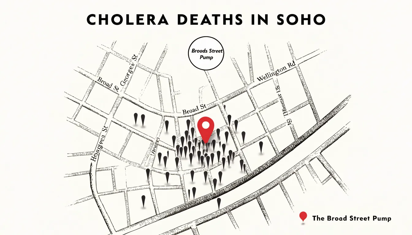
Modern geographic information systems (GIS) carry this tradition forward at vastly greater scale, layering demographic, environmental, and economic datasets onto digital basemaps so that analysts can detect localized disparities and track regional trends. Whether used to display election results by district, visualize the spread of a pandemic, or chart customer concentrations across a territory, maps show how location shapes data.
Statistical Maps
Statistical maps combine geographic boundaries with demographic data to show how people and resources are distributed across space. They rely primarily on two techniques:
- Choropleth maps: One of the earliest and most enduring forms, the choropleth shades predefined administrative regions—such as counties, states, or countries—according to a metric like population density, income level, or literacy rate. Assigning colors or patterns to these areas allows viewers to compare regions at a glance and identify clusters of affluence or deprivation.
- Dot-density maps: This method places individual dots within geographic boundaries, with each dot representing a fixed number of people or events. Rather than averaging values across entire administrative units, dot-density maps preserve the underlying distribution, revealing urban cores, rural sparsity, and fine-grained settlement patterns that choropleths can obscure.
Together, these map types enable analysts to explore socioeconomic phenomena such as the geographic concentration of poverty or the correlation between environmental factors and health outcomes, supporting evidence-based decisions in public health, urban planning, and social policy.
Flow Diagrams
Flow diagrams give shape to movement, encoding magnitude in width and trajectory in position to show how quantities travel through a system. Unlike pie or bar charts, which freeze a moment in place, flow diagrams show where volume originates, how it divides, and where it disappears. This makes them especially suited to questions of efficiency, attrition, and transformation.
The Sankey diagram, named after nineteenth-century engineer Matthew Henry Phineas Riall Sankey, uses bands of varying width to represent quantities moving between stages of a process. Each band’s thickness is proportional to the volume it carries, allowing the eye to follow a resource from its origin through successive transformations and watch it narrow as losses occur. Sankey’s original application traced the energy efficiency of a steam engine, showing how much heat entered the machine and how much emerged as useful work versus waste. That basic grammar remains useful today in energy accounting, supply chain analysis, and budget tracking.
Alluvial plots extend this visual language to the movement of cohorts across categorical states. Named for the layered sediment carried by rivers, these diagrams map individual entities or populations as they shift between categories over time, with each stream branching and merging as members change status. A cohort of customers might be followed through acquisition channels, subscription tiers, and churn events, the widening and narrowing ribbons revealing where groups accumulate and where they drain away. The result is a portrait of dynamic conversion rather than a static snapshot.
Disease Outbreak Maps
Spatial epidemiology relies on the insight that disease does not spread evenly across a landscape; it clusters, follows routes, and concentrates around specific environmental and social conditions. Building on the template established by John Snow’s 1854 cholera map, public health teams use specialized spatial techniques to track and respond to outbreaks.
When applied to epidemiology, dot-density maps render each case as a discrete point. When individual cases carry attributes such as onset date or patient age, the map becomes a record of transmission over days or weeks, revealing localized hotspots. Heat mapping complements this approach by smoothing case data into gradients of intensity, highlighting broader zones of elevated risk. Vector-borne illnesses benefit particularly from this spatial lens: mapping mosquito or tick populations alongside human case data traces the pathways by which pathogens move through an environment. Today, GIS platforms integrate these case counts with mobility data and environmental variables to model how outbreaks might evolve.
The practical payoff is targeted intervention. When public health teams see precisely where transmission clusters are forming, they can direct vaccination campaigns, deploy vector control measures, and concentrate testing capacity far more efficiently than blanket approaches allow. These maps also give policymakers and the public a shared picture of risk to support coordinated responses.
Timeline Charts
Timeline charts arrange events along a continuous horizontal or vertical axis marked with evenly or proportionally spaced dates. Because the eye naturally follows the line in reading order, timelines communicate chronology and sequence without requiring the viewer to decode complex legends or coordinate systems.
This linear structure serves several distinct applications:
- Historical milestones: A nation’s founding, key legislation, and cultural shifts can be plotted in the order they occurred, allowing patterns of cause and effect to emerge visually.
- Process steps: For a manufacturing workflow or a medical procedure, each step occupies a defined point in time, and the intervals between steps carry meaning about duration and pacing.
- Project phases: A product launch timeline might show research, design, testing, and release as segments along the axis, making dependencies and deadlines legible at a glance.
Designers often vary marker size, color, or label density to encode additional information without abandoning the linear backbone, letting a single chart communicate both when something happened and how significant it was.
Scatter Plots
A scatter plot places one continuous variable along the horizontal axis and another along the vertical, marking each observation as a point where the two values intersect. Tracing back to statistical graphics in the late nineteenth century, this format reveals the relationship between two variables through the shape of the resulting point cloud.
When the cloud slopes upward from left to right, the two variables tend to rise together; when it slopes downward, one tends to fall as the other grows. A tight band of points signals a strong association, a diffuse cloud suggests a weaker one, and a shapeless scatter hints that the variables have little to do with each other.
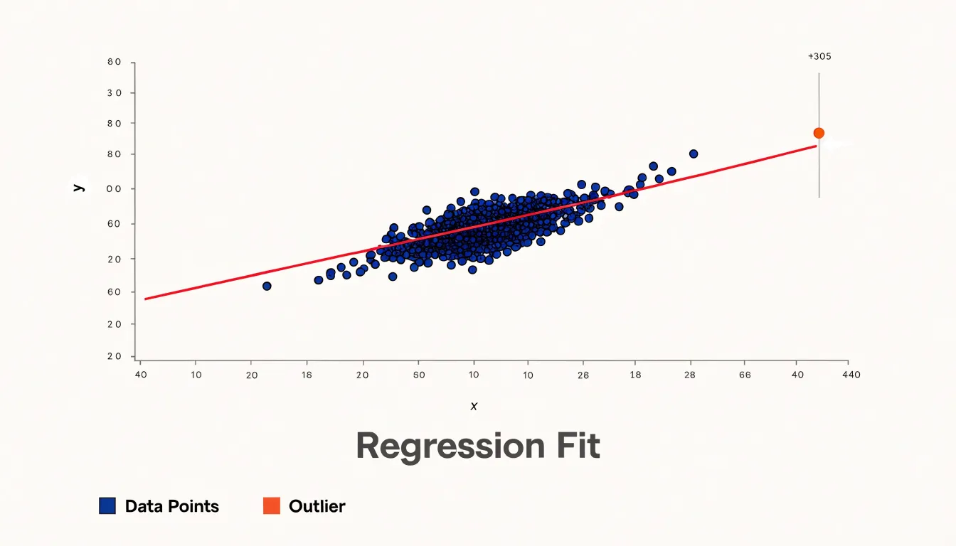
The same coordinate grid exposes exceptional cases. An outlier sitting far from the main cluster stands out at once, whether because its value on one axis is unusually extreme or because it departs from the overall pattern. Identifying these anomalies visually is often faster than scanning tables of numbers, helping analysts spot measurement errors, data entry mistakes, or genuinely unusual phenomena worth investigating.
Scatter plots also serve as a practical check on linear regression models. Once a fitted line is drawn through the points, the analyst can see whether the line captures the underlying trend or whether the data bend away in a curve or spread out in a fan shape, which would violate the model’s assumptions. Points exerting disproportionate influence on the line become visible as well.
Histograms
A histogram converts a column of raw numerical values into a picture of how those values are spread across their range. It divides the full span of the data into a series of contiguous intervals, called bins, and counts how many observations fall into each one. Plotting those counts as adjacent bars approximates the underlying probability distribution of the variable, giving analysts an immediate sense of central tendency, spread, and outliers before formal modeling begins.
The bars sit flush against one another to signal that the variable is continuous rather than categorical, making histograms suited to measurements like heights, incomes, temperatures, or response times. The choice of bin width shapes what the eye perceives: narrow bins expose fine-grained texture and local irregularities, while wider bins smooth the outline to emphasize the broad contour of the distribution.
Once drawn, the bars reveal recognizable distribution shapes:
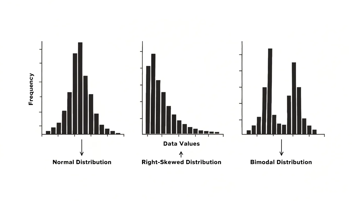
- Normal distribution: A single tall peak with symmetric tails, common in natural measurements.
- Skewness: A long tail stretching to one side, showing that extreme values occur more often in one direction—such as income data piling up at lower values and trailing off toward the wealthy.
- Multi-modal distribution: Two or more distinct peaks, suggesting that the data contains mixed subpopulations, such as measurements pooled from two different groups.
Heatmaps
Heatmaps translate dense numeric tables into a matrix grid where each cell receives a hue whose intensity reflects its stored value. By scanning the color field, a reader can spot bright rows, dark columns, and abrupt transitions that would take minutes to find in a spreadsheet.
In practice, a heatmap condenses several variables at once. Rows might represent products, genes, or web pages, while columns represent months, experimental conditions, or user segments. The color scale encodes a single measured quantity across every combination, highlighting intensity spikes that prompt follow-up questions about why a specific cell or row changed during a given period.
Feature correlations also emerge from the grid. When two columns shade similarly down the length of the matrix, their underlying variables move together; when neighboring rows mirror each other, the observations share behavior. Clustering algorithms often reorder rows and columns to push these similarities into visible blocks, turning a noisy matrix into coherent groups.
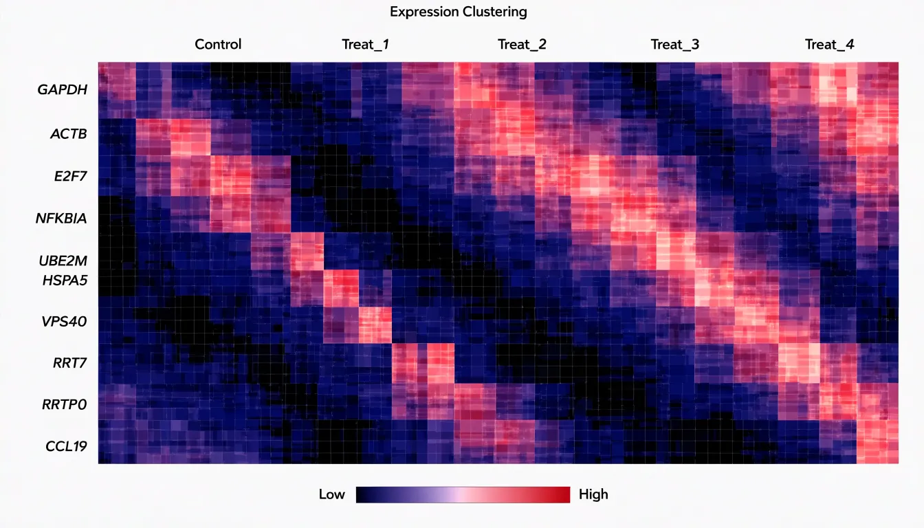
In web analytics and marketing, teams build heatmaps of clicks, scroll depth, or session activity across pages and time slots, or map conversion rates across demographic bands and channels. In each case, the grid turns high-dimensional activity into visible pockets of engagement and clustering.
Tree Diagrams
Tree diagrams give visual form to hierarchical relationships of containment and descent. Their basic grammar consists of nodes (representing entities such as species, departments, or files) and branches (connecting each node to its children). Viewers can trace a path from a single root to any descendant to see where an item sits in the larger order. The branching trees drawn by early naturalists to classify plants and animals remain one of the clearest examples of this structure.
Two specialized forms adapt this hierarchy for different analytical needs:
- Dendrograms: Used in statistical classification and biological taxonomy, dendrograms arrange items along branches whose lengths or joining points encode degrees of similarity. Analysts can see at a glance which observations group together and at what level of the hierarchy those groupings merge.
- Treemaps: Rather than spreading nodes across open branches, treemaps pack hierarchical data into nested rectangles, allocating area in proportion to a quantitative value. Each rectangle subdivides into smaller rectangles for its children, fitting an entire file system, budget, or organizational chart within a single bounded space. This trades the openness of a branching tree for density, letting viewers compare magnitudes across many categories at once.
Network Diagrams
Network diagrams map complex relationship webs by treating entities as nodes and their connections as edges. Each node represents an actor—such as a person, gene, protein, or organization—while each edge encodes a tie like friendship, interaction, or regulatory influence. Directional and weighted edges add further detail by showing who initiates contact or the strength of a bond.
This structure allows analysts to examine two primary properties:
- Structural centrality: Measures like degree, betweenness, and closeness identify nodes in influential positions, revealing hubs that many paths pass through, brokers that bridge separate groups, and peripheral actors with few connections.
- Cluster dynamics: Grouping nodes by connection density exposes distinct communities with tighter internal than external ties. Researchers track how these clusters form, merge, and dissolve over time.
Network visualization grew from hand-drawn sociograms in the 1930s into modern algorithmic layouts—such as force-directed layouts, matrix representations, and interactive tools—capable of rendering thousands of nodes at once. In epidemiology, these diagrams chart contact patterns that shape disease transmission; in molecular biology, they map protein interactions and gene regulatory circuits; and in the social sciences, they expose echo chambers, information brokers, and the spread of influence.
Interactive Graphics
In a static chart, the designer fixes the axes and layers in advance, handing the reader a finished argument. Interactive graphics shift part of that control to the audience, allowing readers to explore the dataset, test hypotheses, and ask their own questions through three core mechanisms:
- User-driven filtering: Sliders, checkboxes, and dropdown menus let viewers isolate a specific region, time period, or demographic category without leaving the page, allowing a single graphic to serve many different inquiries.
- Hovering tooltips: While a static chart shows overall patterns, reading exact values requires squinting at gridlines or consulting a table. Moving a cursor over a mark to reveal precise figures, labels, and context turns the visualization into a lookup instrument as well as a summary, encouraging readers to inspect outliers and individual cases.
- Dynamic zooming: Panning and zooming allow a viewer to move smoothly between a broad overview and fine local detail. A reader might start with a national map, zoom into a single city, and discover a local cluster invisible at the larger scale.
Dashboards
Dashboards bring together real-time metrics, operational key performance indicators (KPIs), and high-level charts into a single interface. By consolidating disparate data streams onto one screen, they allow decision-makers to grasp the state of an organization, process, or market at a glance without compiling reports or waiting for analyst updates.
A well-designed dashboard layers information by urgency and scope. At the top, headline figures and trend charts offer an immediate read on overall health. Below them, operational KPIs break performance down by function, region, or product line so viewers can trace anomalies to their source. Real-time feeds keep these indicators current, making a sudden drop in sales, a spike in server latency, or a shift in customer sentiment visible within minutes rather than weeks later in a quarterly review.
This consolidation shortens the path from observation to action: leaders can spot a deviation, consult supporting charts, and authorize a response within a single session. It also establishes a shared visual vocabulary across teams, shifting conversations from debating whose spreadsheet numbers are correct to deciding what to do next.
Frequently Asked Questions
What are line graphs used for?
Line graphs track change across defined time intervals and reveal trends, rate of change, seasonal fluctuations, and long-term trajectories. They can also compare multiple series over the same interval.
Should I use a bar chart or a pie chart?
Bar charts compare values across categories using length, while pie charts show proportional composition, especially when the number of segments is small and divisions fall into intuitive fractions. Angles are less precise than lengths, so fine distinctions between similar pie slices are hard to judge.
What is the difference between a choropleth map and a dot-density map?
A choropleth map shades predefined administrative regions according to a metric such as population density, income level, or literacy rate. A dot-density map places individual dots within geographic boundaries, with each dot representing a fixed number of people or events, preserving the underlying distribution.
What does a Sankey diagram show?
A Sankey diagram uses bands of varying width to represent quantities moving between stages of a process, with each band’s thickness proportional to the volume it carries. It shows where volume originates, how it divides, and where it disappears, such as losses in energy accounting.
How are maps used to track disease outbreaks?
Disease outbreak maps plot cases, hotspots, and broader zones of elevated risk using techniques such as dot-density maps and heat mapping. Public health teams use them to direct vaccination campaigns, deploy vector control measures, and concentrate testing capacity where transmission clusters are forming.
What can you learn from a scatter plot?
A scatter plot reveals the relationship between two continuous variables through the shape of the resulting point cloud. It can also expose outliers and help check whether a linear regression line captures the trend or whether the data bend away in a curve or fan shape.
Tony Astor
Tony writes about data visualization and the tools people use to build charts and dashboards. More about Data Illustrator